Topology

Building on the available deﬁnitions, additional structures can be introduced, which can be described as being the bones of geometry as well as being useful for programming abstractions.

Deﬁnition 28 (Topology) A topology $𝒯$ of a set $𝒳$ is deﬁned by the following properties:

-: Both $∅∈𝒯$ and $𝒳 ∈ 𝒯$ .
-: A ﬁnite intersection of members of $𝒯$ is in $𝒯$ .
-: An arbitrary union of members of $𝒯$ is in $𝒯$ .

The concept of a topology alone is incomplete, when not applied to a set, thus providing:

Deﬁnition 29 (Topological space) The pair of the set $𝒳$ and the topology $𝒯$ are denoted as the topological space $(𝒳 ,𝒯 )$ .

Topological spaces also allow to further qualify the concepts of mappings, as provided by Deﬁnition 20.

Deﬁnition 30 (Continuous mapping) A mapping between two topological spaces

ϕ : (𝒳 ,𝒯X ) → (𝒴, 𝒯Y ) (4.33)

is continuous, if the preimages of open sets are open sets.

Equipped with the concept of continuity it is beneﬁcial to specially label a certain class of continuous, invertible mappings.

Deﬁnition 31 (Homeomorphism) A continuous mapping $ϕ$ is called a homeomorphism or topological isomorphism, if it satisﬁes the following properties:

$ϕ$ is a bijection
the inverse mapping $ϕ− 1$ is also continuous

Beside continuity (Deﬁnition 30), relations between two mappings from a topological space to another are of interest. Special requirements in this regard are encountered for example in Deﬁnition 39, thus motivating the following deﬁnition.

Deﬁnition 32 (Homotopy) Given two continuous mappings $f : 𝒜 → ℬ$ and $g : 𝒜 → ℬ$ , a homotopy $h$ is a continuous mapping such that:

h : 𝒜 × [0;1 ] → ℬ such that (4.34a) 𝒜 × {0 } : h(x,0) = f(x ) (4.34b) 𝒜 × {1 } : h(x,1) = g(x) (4.34c)

Further reﬁnement of the concept of a topological space (Deﬁnition 29) by including separability of neighbourhoods of diﬀerent elements of the topological space allows to move closer to the desired settings of geometry described in Deﬁnition 37.

Deﬁnition 33 (Hausdorﬀ spaces) The topological space $(𝒳 ,𝒯 )$ is called Hausdorﬀ, if

∀x,y(x ⁄= y ) ∈ 𝒳 (4.35)

there exist open sets $U1, U2$ such that 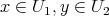$x ∈ U1,y ∈ U2$ and $⋂ U1 U2 = ∅$ .

From the concept of a Hausdorﬀ space an important deﬁnition can be derived, which is invaluable for use in the discrete settings of digital computers:

Deﬁnition 34 (CW Complex) The pair of a Hausdorﬀ space $X$ (Deﬁnition 33) together with a decomposition $E$ , whose elements $e ∈ E$ are called cells, is a CW complex, if the following criteria are met:

The interior of every cell $e ∈ E$ can be mapped continuously (Deﬁnition 30) to an open ball.
Every closed cell is contained in a ﬁnite union of open cells.
A subset $A ⊂ X$ is open if and only if $∀e ∈ E, A ∩ e$ is open.

A further intermediate deﬁnition is introduced, before arriving at the topological space, which carries suﬃcient additional structure to accommodate the geometric entities (e.g., Deﬁnition 54). It serves to again partition the requirements into manageable components, so as not to end up with overly complex and contorted constructs.

Deﬁnition 35 (Topological manifold) A topological manifold $𝔐$ of dimension $n$ is a Hausdorﬀ space which is locally homeomorphic to $ℝn$ . Consequently, this results in the existence of bijective mappings $κ$ , called charts, of the form

n κ : 𝒰 → ℳ ⊆ ℝ , (4 .36)

which map open neighbourhoods $𝒰$ for every element $p ∈ 𝔐$ to open subsets $n ℳ ∈ ℝ$ . The $n$ -tuple of numbers resulting from $κ (p )$ is called the (local) coordinates of $p$ .

As the subsets $𝒰$ are open and the charts operate solely on them, any conclusion from a single chart alone must remain a local one. However, open subsets may be combined to overcome this limitation thus giving rise to:

Deﬁnition 36 (Atlas) A collection of charts forming an open cover (Deﬁnition 1)

⋃ 𝒜 = (𝒰i,κi) (4.37) i

is called an atlas $𝒜$ .

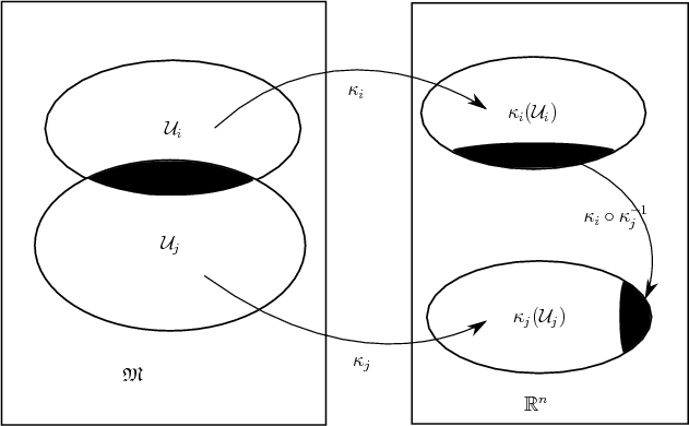
Since the atlas is now deﬁned on the whole manifold, it is possible to judge global properties. Considering two charts of an atlas $κ (𝒰 ) ∈ 𝒜 i i$ and $κ (𝒰 ) ∈ 𝒜 j j$ with the non-empty intersections of open sets

Figure 4.1: Chart transitions on a manifold.

The following deﬁnition ﬁnally introduces a topological space, which is equipped to admit the diﬀerential structures required in the further geometrical considerations (Deﬁnition 48).

Deﬁnition 37 (k-Diﬀerentiable manifold) A topological manifold $𝔐$ with an atlas $𝒜$ is called a diﬀerentiable manifold, if the transitions between charts $∀κ ∈ 𝒜$ are of diﬀerentiability class $k C$ .

The requirement of diﬀerentiable transitions between mappings relies on the charts themselves being homeomorphisms (Deﬁnition 31) as continuity is a prerequisite for diﬀerentiability. The additional structure of a diﬀerentiable manifold also allows to place a more stringent requirement on a homeomorphism, which is expressed in the following deﬁnition.

Deﬁnition 38 (Diﬀeomorphism) A homeomorphism (Deﬁnition 31), which is itself diﬀerentiable as well as its inverse, is called a diﬀeomorphism.

Diﬀerentiable manifolds and diﬀeomorphisms are of particular importance for physical applications, as already attributed by the ancient adage “natura non facit saltus”.

4.4 Topology