Boltzmann’s Equation in Integral Form

5.6 Boltzmann’s Equation in Integral Form

Starting with Boltzmann’s equation in diﬀerential form

dρ ∂ρ ---= ---+ {ρ, H } = Q (ρ ), (5 .41) dt ∂t

it is seen that the evolution of the system is connected to the Hamiltonian deﬁned on the phase space. Test particles evolve on trajectories (Deﬁnition 45), which comprise the Hamiltonian ﬂow corresponding to the Hamiltonian vector ﬁeld (Deﬁnition 62). Thus trajectories are essential to determine the evolution connected to Boltzmann’s equation.

In addition to the trajectories, which are deﬁned by the geometry of the phase space via the Hamiltonian $H$ , it is also required to give a speciﬁc description of the collision operator on the right hand side. In the ﬁeld of semiconductor simulations it is common to describe the collision operator $Q (ρ)$ in the form

∫ ′ ′ ′ ′ Q(ρ ) = S (p ,p, q)ρ(p ,q,t) − S(p, p ,q)ρ(p,q, t)dp . (5.42)

Using the concept of trajectories on which particles travel, the two components of this integral expression can be interpreted to have physical signiﬁcance. The ﬁrst component of the given integral describes the loss of particles on a given trajectory due to collision/scattering events to other trajectories, thus called out-scattering. The second part models the gains to this particular trajectory due to the collision/scattering mechanisms, aptly called in-scattering. This second term can be simpliﬁed by setting

∫ S (p,p ′,q )dp ′ = λ(p,q ). (5.43)

Thus Equation 5.42 becomes

∫ ′ ′ ′ Q (p,q, t) = S(p ,p, q)ρ(p ,q,t)dp − λ(p,q )ρ(p,q, t). (5.44)

As already indicated the evolution is inherently linked to trajectories $γ$ in phase space which provide a mapping of a curve parameter to the phase space points, represented by the pair $p$ , $q$ .

∗ γ : ℝ → T M (5.45a) γ (r) → (p,q ) (5.45b)

As such the expression for $λ (p, q)$ can also be rendered as $λ(r)$ as a short form for

λ (r ) = λ (γ(r)) = λ(p,q ), γ(r) = (p,q ). (5.46)

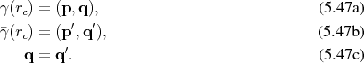
$γ(r)$ represents the trajectory travelled before a scattering event, while the particle continues to travel on a trajectory $¯γ(r)$ as indicated in Figure 5.3 afer a scattering event. With the two curves requiring to match at the parameter $r c$ corresponding to a collision/scattering event in the following manner

γ (rc) = (p, q), (5.47a) γ¯(rc) = (p ′,q′), (5.47b) ′ q = q . (5.47c)

Utilizing these settings, Equation 5.42 can be rendered as

∫ dρ(γ(t)) ′ ′ ′ dt + λ(γ(t))ρ (γ (t)) = S(p ,γ(t))ρ(p ,q,t)dp = (5.48a) ∫ dρ(γ(t))+ λ(γ(t))ρ (γ (t)) = S(¯γ (t),γ(t))ρ(¯γ(t))dp′. (5.48b) dt

In the following the dependence of the curves $γ$ on the parameter shall be suppressed, where it facilitates readability without adversely aﬀecting clarity.

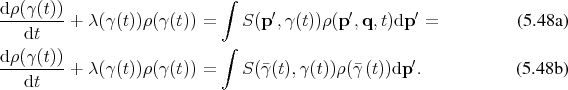
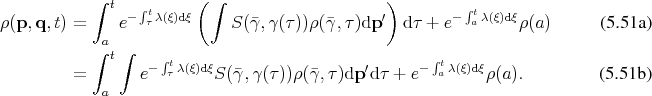
Here it is desirable to ﬁnd an integrating factor, so that the left hand side resembles a total derivative. The integrating factor in this case is

∫ τ e− t λ(ξ)dξ, (5 .49)

as can easily be veriﬁed by simple diﬀerentiation.

d ( − ∫τ λ(ξ)dξ ) − ∫τλ(ξ)dξ ∫ ′ --- e t ρ(γ, t) = e t S (¯γ,γ)ρ(¯γ)dp (5.50) dt

Applying deﬁnite integration the expression for the solution of Boltzmann’s equation becomes

∫ (∫ ) t − ∫τtλ(ξ)dξ ′ − ∫taλ(ξ)dξ ρ(p,q,t) = e S (γ¯, γ(τ))ρ(¯γ,τ)dp dτ + e ρ(a) (5.51a) ∫at∫ ∫ ∫ = e− tτ λ(ξ)dξS (¯γ, γ(τ))ρ(¯γ,τ)dp ′d τ + e− taλ(ξ)dξρ(a). (5.51b) a

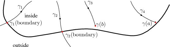
The last term deserves special consideration. It is easy to argue that it represents the initial conditions of the sought function from which the system begins to evolve. It however also accommodates boundary conditions as becomes apparent, when considering that the points of the trajectories corresponding to the parameter $a$ not necessarily lie within the domain of interest. In this case the trajectory within the domain uses the value at the boundary instead as illustrated in Figure 5.4. Thus the term accommodates both, initial as well as boundary conditions for this integral equation [92].

PICT

Figure 5.4: Trajectories accommodate initial as well as boundary conditions.