Statistical Description – Boltzmann’s Equation

5.4 Statistical Description – Boltzmann’s Equation

So far little heed was paid to the number of entities under consideration as the formalisms are abstract enough to deal with a scaling of the degrees of freedom. When considering $N$ identical but distinct entities in a three-dimensional setting, the associated phase space is simply a Cartesian product (Deﬁnition 3) of the single phase spaces, thus forming an overall space of dimension $6N$ . While the formalism does not hinder the speciﬁcation of problems encompassing multiple entities, it becomes increasingly diﬃcult to obtain solutions. Furthermore, when turning to systems composed of particularly large numbers of entities, such as molecules or atoms in gases, it becomes quite unfeasible to deal with them directly, as the sheer amount of boundary and/or initial conditions becomes prohibitive.

Therefore, a description oﬀering a reduction of the overwhelming degrees of freedom is called for. This can be demonstrated using a basic equation describing the evolution of $N$ particles using a density depending on the $N$ phase space coordinates and time

∗ N ρ (z1,...,zN ,t) : T M × ℝ → ℝ zi = (q,p ) (5.32)

and a Hamiltonian $H$ , which depends on all of the particles.

H : T ∗M N → ℝ (5.33a) ∂ρ ---+ { ρ,H } = 0 (5.33b) ∂t

By averaging by means of integration (Deﬁnition 94) an $n$ particle distribution function is obtained

∫ ρn(z1,...,zn,t) = ρ(z1,...,zN,t)dzn+1 ...dzN, n < N, (5 .34)

thus constructing a projection (Deﬁnition 25)

∗ N ∗ n π : T M → T M (5.35)

such that the higher-dimensional phase space $N T∗M$ appears as a ﬁber (Deﬁnition 40) over the reduced phase space $T∗M n$ , since it is certain that

T∗M N = T ∗M n × T∗M (N −n), (5 .36)

An equation governing the evolution of this reduced density function can be obtained by integrating Equation 5.33b, resulting in the expression

∫ ∂ρn-+ {ρn, Hn} = (N − n ) ˙pnρn+1dzn+1 (5.37) ∂t

where the left hand side containing the Hamiltonian $H n$ depends on the considered $n$ particles, while the right hand side describes the interactions with all the remaining $N − n$ particles by coupling to the next higher distribution function. Therefore this equation is not closed, but gives rise to a hierarchy of equations, the BBGKY, named after the individuals who have independently derived this system, Bogoliubov [87], Born [88], Green [89], Kirkwood [90] and Yvon [91 ].

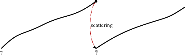
Using this formulation, the restriction to just one particle yields an expression for a single particle Hamiltonian, which results in phase space trajectories with deviations from these trajectories attributable to collisions.

∂ρ --1-+ {ρ1,H1 } = Q (ρ1) (5.38) ∂t

This also shows the price which has to be paid for the reduction of degrees of freedom. The observed particle will no longer follow a simple curve through phase space and is disturbed due to the scattering term which appears on the right hand side as is illustrated in Figure 5.3.

Figure 5.3: The trajectory is interrupted due to scattering.

While the derivation naturally describes the collison term with other particles, it can also model the interaction of the particle tracked by Boltzmann’s equation with the envrionment, thus allowing for an interpretation as probability of a particle evolving to a given point.

While Boltzmann’s equation appears as a simpliﬁcation here, it is far from easy to obtain solutions to this deceivingly simple equation. Therefore several diﬀerent techniques have been developed to at least calculate estimates in diﬀerent contexts and with various levels of accuracy.