In this chapter the application of the level set and fast marching methods for the development and implementation of the topography simulator ELSA in two and three dimensions is presented. ELSA rest on many techniques, including a narrow band level set method, fast marching for solving the Eikonal equation and extension of the speed function, transport models, visibility determination, and an iterative equation solver.
The development and implementation of a two-dimensional topography simulator based on the level set method have begun at our institute by Dr. Heitzinger [35]. It has been written in Lisp. However, its use was only limited to the simulation of the deposition of layers into single features.
Every feature-scale topography simulation must take the following three main steps into account. First, the transport of particles above the wafer in the boundary layer must be simulated. This can happen in the radiosity regime as described in Section 5.3. Second, the fluxes of particles at the wafer surface found in the previous step determine the chemical reactions that take place at the wafer surface. Third, the surface of the substrate moves according to the fluxes found in the second step.
 |
In order to apply the level set method a suitable initial function
![]() has to be determined first. There are two requirements:
first it goes without saying that its zero level set has to be the
surface given by the application, and second it should essentially be
a linear function so that linear
interpolation can be applied in the final surface extraction step.
has to be determined first. There are two requirements:
first it goes without saying that its zero level set has to be the
surface given by the application, and second it should essentially be
a linear function so that linear
interpolation can be applied in the final surface extraction step.
The signed distance function of a point from the given surface has
shown to be a good choice for the initial level set function. This function is the common distance function multiplied by minus or plus one depending
on which side of the surface a grid point lies. The common distance
function of a point ![]() from a set
from a set ![]() is then defined by
is then defined by
![]() , where
, where ![]() is a metric, usually the Euclidean
distance.
is a metric, usually the Euclidean
distance.
Consider a fixed orthogonal grid for a whole simulation
domain. Because of the ease of two-dimensional illustration, we
show a two-dimensional interface introduced as
a series of points which form line segments. To construct the
initial boundary, we try to keep
the number of points representing the interface to a minimum to avoid long
computational time during the calculation of the initial level set
function. Figure 5.2 shows an example to illustrate
the technique used for the calculation of a common distance function. Consider the
grid point ![]() whose distance from the boundary we want to calculate. We first calculate the distance of
whose distance from the boundary we want to calculate. We first calculate the distance of ![]() from all segments
which form the boundary. The line segments are
from all segments
which form the boundary. The line segments are ![]() ,
, ![]() ,
, ![]() ,
, ![]() ,
and
,
and ![]() . From elementary mathematics we know that the distance of a
point from a line is the length of the normal line drawn from point to the
line, e.g., the distance of
. From elementary mathematics we know that the distance of a
point from a line is the length of the normal line drawn from point to the
line, e.g., the distance of ![]() from line segment
from line segment ![]() is
is
![]() . However, there is not always an intersection point between the
normal line and segment as it is the case for the line segment
. However, there is not always an intersection point between the
normal line and segment as it is the case for the line segment ![]() , where
, where
![]() is outside
is outside ![]() . In such cases the distance is the minimum of
. In such cases the distance is the minimum of
![]() and
and ![]() .
.
![\includegraphics[width=0.75\linewidth]{figures/initial2}](img226.png)
|
After the calculation of these different distances and
getting the minimum value among them, we still need to assign a sign to
this value depending on the position of the grid point relative to the boundary. In
order to do this we choose a reference point ![]() inside the boundary and
at the bottom of the simulation domain. If the connection line between
a grid point and the reference point intersects the boundary at an odd
or even number of times, the grid point is outside or inside the
boundary and the common distance function must be multiplied by plus or
minus one, respectively. For example, the grid point
inside the boundary and
at the bottom of the simulation domain. If the connection line between
a grid point and the reference point intersects the boundary at an odd
or even number of times, the grid point is outside or inside the
boundary and the common distance function must be multiplied by plus or
minus one, respectively. For example, the grid point ![]() is outside
the boundary since the line
is outside
the boundary since the line ![]() intersects the boundary once at
intersects the boundary once at
![]() and the grid point
and the grid point ![]() is inside the boundary, because the line
is inside the boundary, because the line ![]() intersects the boundary twice, at
intersects the boundary twice, at ![]() and
and ![]() .
.
Since the level set algorithm will later only work in a narrow band
and the calculation of the distance function
especially in three dimensions is very CPU expensive, it is sufficient to perform the distance
calculations near the initial boundary. This can be achieved, e.g., by
a recursive algorithm walking along the boundary. First, a point
whose distance to the boundary is smaller than the width of the future
narrow band is identified by walking along the boundary of the simulation
domain in ![]() -direction or
-direction or ![]() -direction for two or three dimensions,
respectively. When such a point is found, it is used as
the starting point for the recursion. In the recursion only points
with a distance smaller than the narrow band width are considered for the
next step. The maximum distance ever computed during this procedure
is used to initialize the grid points above and below the boundary
with a positive or negative sign, respectively. This method reduces the computational effort of initialization from
-direction for two or three dimensions,
respectively. When such a point is found, it is used as
the starting point for the recursion. In the recursion only points
with a distance smaller than the narrow band width are considered for the
next step. The maximum distance ever computed during this procedure
is used to initialize the grid points above and below the boundary
with a positive or negative sign, respectively. This method reduces the computational effort of initialization from
![]() and
and ![]() to
to ![]() and
and ![]() in three and two
dimensions, respectively, where
in three and two
dimensions, respectively, where ![]() is the number of grid points in each
direction.
is the number of grid points in each
direction.
For three-dimensional initialization, in analogy to two dimensions one has to calculate the
distance of the grid points to different triangles which represent the
boundary. The distance of a point from a
triangle ![]() is given by
is given by
![]() and the
distance
and the
distance ![]() of a point from the initial boundary
of a point from the initial boundary
![]() , consisting of a set of triangles, is given by
, consisting of a set of triangles, is given by
![]() .
.
![\includegraphics[width=\linewidth]{figures/distancefunction}](img239.png)
|
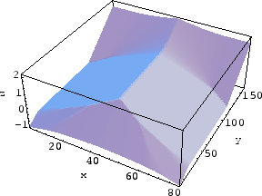
The initial level set function for a rectangular trench is shown in Figure 5.3. As it can be seen in this figure the signed distance function is a linear function with a value of zero at the boundary.
Before we begin to describe the radiosity model used by transport of particles, we have to present the definition of the visibility of a point from another point. This plays an important role for the calculation of the flux at the surface elements as it can be seen later in this section.
Figure 5.4 is an illustrative example
for the definition of visibility. There are different kinds of visibility
which have to be defined. The first kind is the visibility among the
points of a boundary such as ![]() ,
, ![]() , and
, and ![]() . The second kind
is the visibility between a boundary point and a source point which is
assumed to be
. The second kind
is the visibility between a boundary point and a source point which is
assumed to be ![]() in Figure 5.4. Whereas the pairs of points
in Figure 5.4. Whereas the pairs of points ![]() ,
, ![]() ,
,
![]() , and
, and ![]() are
visible from each other, there is no visibility between the pairs of
points
are
visible from each other, there is no visibility between the pairs of
points ![]() and
and ![]() .
.
A formulation of the radiosity model [80] for the case of luminescent reflection, pertaining to low energy particles (cf. Section 4.1), can be used in the deposition simulations.
To model deposition it is assumed that the distribution of the particles coming from the source obeys a cosine function around the normal vector of the plane in which the source lies [19]. This implies that the incoming flux at a surface element is proportional to the cosine of the angle between the connecting line between the center of mass of a surface element and the source, and the normal vector of the source plane.
The flux reaching the surface elements obtained by the surface extraction step may be written as a vector,
 |
![$\displaystyle \Psi_{ij} = \frac{n_i\cdot(t_j-t_i) n_j\cdot(t_i-t_j)}{\pi \vert t_j-t_i\vert^3}v_{ij}
%[\mbox{$i$ visible $j$}]
$](img250.png)
The second line in the equation above is obtained from the first one
and the relationship
![]() results from straightforward algebraic manipulations. In the case of
multiple, low energy species, the calculation of the visibility matrix
and the inverse
results from straightforward algebraic manipulations. In the case of
multiple, low energy species, the calculation of the visibility matrix
and the inverse ![]() only depends on topographic information and thus does
not have to be repeated for each species.
only depends on topographic information and thus does
not have to be repeated for each species.
Most of the computation time for the simulation of the transport of
the particles above the wafer by the radiosity model is consumed by first
determining the visibility between a surface element and
the source, and secondly, between two different surface elements. The latter has an
![]() operation complexity, where
operation complexity, where ![]() is the number of surface elements growing
approximately with
is the number of surface elements growing
approximately with ![]() . If the connecting line between the center of mass of two surface
elements does not intersect the surface, i.e., the zero level set, those
surface elements are visible from each other. In order to decrease the
computational effort related to determining the visibility between
the surface triangles, we have assumed that two triangles are visible
from each other if the center point of the grid cells in which the
triangles are located, are visible from
each other. Since there are at least two triangles in each grid cell,
considerable time is saved.
. If the connecting line between the center of mass of two surface
elements does not intersect the surface, i.e., the zero level set, those
surface elements are visible from each other. In order to decrease the
computational effort related to determining the visibility between
the surface triangles, we have assumed that two triangles are visible
from each other if the center point of the grid cells in which the
triangles are located, are visible from
each other. Since there are at least two triangles in each grid cell,
considerable time is saved.
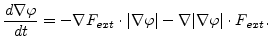
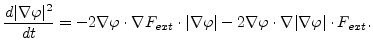
After we have calculated the speed function on the boundary, where the models of calculation differ depending on the process conditions (in Chapter 4 we will introduce several different models which are used to calculate the speed function on the boundary), we can start with extending the speed function. An extended speed function must satisfy two basic requirements. First it has to match the speed function calculated from a physical model on the boundary, and second it has to guarantee that it moves the other level sets in such a way that the signed distance function is preserved.
Assume that
![]() is a signed distance function which satisfies
is a signed distance function which satisfies
![]() . We will prove that
. We will prove that
![]() will be equal to one, i.e., the level set function remains a signed distance
function, if we build the following equation to extend the
speed function [104]
will be equal to one, i.e., the level set function remains a signed distance
function, if we build the following equation to extend the
speed function [104]
Now the speed function can be extended. For a level set function
![]() , where
, where ![]() stands for the
stands for the ![]() th time step, we
choose a signed distance function
th time step, we
choose a signed distance function
![]() whose zero level set
is equal to the zero level set of
whose zero level set
is equal to the zero level set of
![]() . As mentioned above,
we need to satisfy the following equation
. As mentioned above,
we need to satisfy the following equation
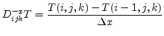
The upwind scheme5.1 of
(5.5) enables the calculation of ![]() from the grid points
adjacent to the boundary which have the smallest values of
from the grid points
adjacent to the boundary which have the smallest values of ![]() . The boundary is swept along considering points
in a narrow band (cf. Section 5.6) around the
boundary. Marching this narrow band forward and freezing the values of
the existing points and bringing the new points into the narrow band
results in a solution of the Eikonal equation within the narrow
band. More details can be found in [78,79].
. The boundary is swept along considering points
in a narrow band (cf. Section 5.6) around the
boundary. Marching this narrow band forward and freezing the values of
the existing points and bringing the new points into the narrow band
results in a solution of the Eikonal equation within the narrow
band. More details can be found in [78,79].
One technique to reduce the calculation time is to use adaptive mesh refinement. This refinement may be required especially in two regions. The first region is where the curvature of the boundary is high and the second is where the speed function changes very rapidly. For example, if the zero level set identified with the boundary is the object of interest, as is normally the case, then one has to adaptively refine the mesh around the location. However, considerable care must be taken at the interfaces between the fine and coarse cells. In particular, a subtle update strategy for the level set function values is required at so called hanging nodes where the boundary between two levels of refinement does not have a full set of nearest neighbors. Whereas advection terms which do not depend on the curvature lead to hyperbolic equations and a straightforward interpolation of the level set values from the coarse grid points easily produces the level set values at hanging nodes, there are some complications for the curvature dependent advection terms. The situation is not so straightforward, since this corresponds to a parabolic term that can not be approximated by simple interpolation [80].
The idea leading to fast level set algorithms stems from the observation that only the values of the level set function near its zero level set are essential, and thus only the values at the grid points in a narrow band around the zero level set have to be calculated. The advantages of this technique are as follows:
![\includegraphics[height=13.5cm]{figures/bestformn.eps}](img286.png)
|
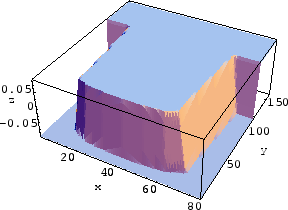
Figure 5.5 shows the simulation results of different
steps of a deposition process into a typical trench. Except for step 0 for which the level set function
with and without narrow banding has been shown, other
intermediate level set functions corresponding to
Figure 5.5 have been shown only within the narrow
band in Figure 5.6. The grid resolution is
![]() . The zero level set can be seen easily in each intermediate step and
the formation of a void in step 48, as well.
. The zero level set can be seen easily in each intermediate step and
the formation of a void in step 48, as well.
|
[Step 0 without narrow banding]
 [Step 0]
 [Step
[Step  [Step
[Step 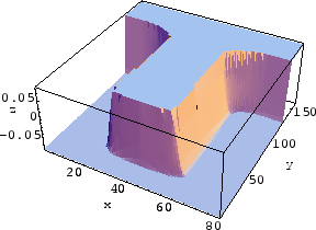 [Step
[Step 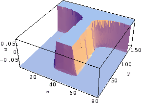 [Step
[Step 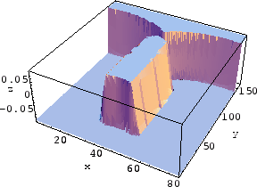
|
In this section we present the implementation of an algorithm which combines narrow banding and extension of the speed function. This algorithm works as follows: first the initial points near the zero level set, where the speed function is known, and the neighboring trial points are determined. It is checked in the main loop, if there still is a trial point to be considered in the narrow band. All trial points are stored on a heap ordered by their distance from the zero level set. If there is a point to be considered, its distance is approximated, its extended speed is calculated, and its neighbors are updated accordingly. Finally, after the main loop, the bookkeeping information for the narrow band points is updated using the distance information just computed.
The detailed steps using several auxiliary functions are as follows: concerning the data structures, the information about the level set grid, the distance function, the extended speed function, and the tags for the fast marching method are stored in arrays. The trial points are stored on a heap. The implementation flow is as follows:
Hence it is mandatory to keep the number of surface elements as low as possible. However, decreasing the number of surface elements must be done in such a way that the high resolution is obtained where it is needed, e.g., near the trench opening and at the bottom of the trench. One approach is to devise a refinement and coarsening strategy for unstructured grids at the level set implementation and the algorithms working on it. This, however, complicates the implementation because of the complex fast marching algorithm necessary at the unstructured grid compared to the algorithm at the rectangular grid which is used normally for the implementation of the level set method. In this work a different approach was taken by coarsening the surfaces after they have been extracted from the level set grid.
The coarsening algorithm works by walking down the list of surface
elements extracted as the zero level set and calculating the
angle between two neighboring surface elements. Whenever
this angle is below a certain threshold value of a few degrees,
the neighboring elements are coalesced into one. After one sweep
through the list, the algorithm can be reapplied for further
coarsening. After ![]() coarsening sweeps, at most
coarsening sweeps, at most ![]() surface
elements are coalesced into one. The resulting longer surface
elements are used for the radiosity calculation, after which the
fluxes are translated back from the coarsened elements to the original
ones. This is a heuristic approach and has shown excellent results.
surface
elements are coalesced into one. The resulting longer surface
elements are used for the radiosity calculation, after which the
fluxes are translated back from the coarsened elements to the original
ones. This is a heuristic approach and has shown excellent results.
To discretize the level set equation, one can substitute the time
and spatial derivatives with forward and central differences,
respectively. We now consider a boundary with a right angle at the corner that
is moved with a constant speed function normal to the boundary. Studies in
[80,35] have shown that using the central differences for spatial
derivatives leads to false values of the gradient at the corner
point. Since the slope
![]() is not
defined at corners, the central difference approximation sets it to
the average of the left and right slopes. Therefore, this wrong
calculation of the slope propagates away from the corner and leads to
oscillations.
is not
defined at corners, the central difference approximation sets it to
the average of the left and right slopes. Therefore, this wrong
calculation of the slope propagates away from the corner and leads to
oscillations.
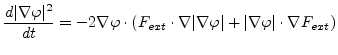
An alternative approach would be to add a viscosity term to the right hand side of the level set equation as follows [80]:
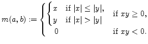
The best approach to discretize the equations of the form
![]() are the following space convex schemes,
where it is assumed that the flux
are the following space convex schemes,
where it is assumed that the flux
![]() is convex, i.e.,
is convex, i.e.,
![]() [80]. These approaches ensure that discontinuities and
boundaries remains sharp.
[80]. These approaches ensure that discontinuities and
boundaries remains sharp.
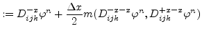
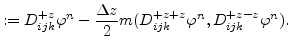
The simplest scheme to discretize the level set equation is the first order space convex scheme which is as follows:
| (5.6) |
![$\displaystyle \max(D^{-z}_{ijk}\varphi ^{n},0)^{2}+\min(D^{+z}_{ijk}\varphi ^{n},0)^{2}\Bigl]^{\frac{1}{2}}$](img312.png) |
![$\displaystyle \max(D^{+z}_{ijk}\varphi ^{n},0)^{2}+ \min(D^{-z}_{ijk}\varphi ^{n},0)^{2}\Bigl]^{\frac{1}{2}}.$](img315.png) |
For the second order space convex scheme
![]() and
and
![]() are defined as follows:
are defined as follows:
 |
||
 |
||
 |
||
 |
||
 |
||
 |
This scheme takes care of shocks by building an appropriate switch. A comparison between these two different schemes can be found in [35].
As mentioned in Section 5.3 the radiosity model assumes that the total flux depends on the flux directly from the source, as well as an additional flux due to the particles which do not stick and are re-emitted. After discretizing the problem the flux vector whose elements are the total flux at different surface elements can be expressed by a matrix equation.
There are two numerical approaches to solve this equation. The first is to use a direct solver for the matrix equation. Although this is practical in two dimensions [13,14,11], it becomes impractical due to the computational effort needed to calculate the inverse matrix for three-dimensional problems. In three dimensions the equation is solved iteratively.
The iterative solution developed by Adalsteinsson and Sethian [80] consists of a series expansion of the radiosity matrix. Suitably interpreted, it can be viewed as a multi-bounce model in which the number of terms in the series expansion corresponds to the number of bounces that a particle can undergo before its effect is negligible.
The iterative solution allows one to check the error term to determine how many terms must be kept. Since most of the particles either stick or leave the domain after a reasonable number of bounces, this is an efficient approach.
The reflected intensity after the ![]() -th bounce is defined as
-th bounce is defined as
![]() . The relationship between reflected intensity and source
intensity at the
. The relationship between reflected intensity and source
intensity at the ![]() -th surface element is written (cf.
Section 5.3) as follows:
-th surface element is written (cf.
Section 5.3) as follows:
| (5.7) |
In matrix form, this becomes
| (5.8) |
| (5.9) |
Now ![]() is defined to be the portion that sticks after the
is defined to be the portion that sticks after the ![]() th
bounce.
th
bounce.
| (5.11) |
In general,
 |
(5.12) |
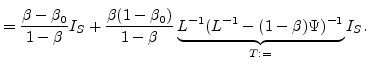
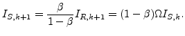
Therefore, by going back to the initial expression (5.10)
| (5.13) |
![$\displaystyle I_{N}=\beta(1-\beta_0)\Bigl[\sum_{k=1}^{N}(1-\beta)^{k-1}\Omega^{k}\Bigl]I_{S} + \beta_0 I_{S}.$](img340.png) |
(5.14) |
Each application of the operator may be viewed as either an additional
term in the expansion or an additional included bounce. It is
important to note that there is a recurrence relation for ![]() given by
given by
![$\displaystyle I_{N+1}=\beta(1-\beta_0)\Bigl[\sum_{k=1}^{N+1}(1-\beta)^{k-1}\Omega^{k}\Bigl]I_{S}+\beta_0 I_{S}$](img341.png) |
(5.15) |
![$\displaystyle I_{N+1}=\beta(1-\beta_0)\Bigl\{(1-\beta)\Omega\Bigl[\sum_{k=1}^{N}(1-\beta)^{k-1}\Omega^{k}\Bigl]+\Omega\Bigl\}I_{S}+\beta_0 I_{S}$](img342.png) |
(5.16) |
| (5.17) |
| (5.18) |
By constructing the remainder term
![]() , the convergence of
the expansion can be measured and sufficient terms can be kept to bound the error below a
user-specified tolerance.
, the convergence of
the expansion can be measured and sufficient terms can be kept to bound the error below a
user-specified tolerance.
Three-dimensional ELSA requires a library called IPD (input deck library) developed by the Institute for Microelectronics [51]. It is used for parsing input files and must be installed first. An example of an IPD input file including parameters of the simulator, process parameters, and the initial geometry is as follows:
Simulation
{
  Name = "Sample";
  Comment = "a sample deposition with void";
  OutputDirectory = "./output/";
  WriteAfterEachIteration = "yes";
  PrintConfig = "short";
}

// Parameters of the level-set algorithm
LevelsetAlgorithm
{
  nx=30;
  ny=30;
  nz=30;
}

Sources
{
  SourceGroup1
  {
    z = 2.0;
    x1 = 0.0;
    y1 = 0.0;
    x2 = 1.0;
    y2 = 1.0;
    xSourceCount = 4;
    ySourceCount = 4;
    Intensity = 20;
    n = 1;
    Direction = [0,0,-1];
  }
}

Steps
{
  Deposition1
 {
    Name = "Deposition1";
    Material = "Si3N4";
    Time = 8.0;
    MaxThickness = 0.23;
    SourceStickingProbability = 0.1;
    ReflectionStickingProbability = 0.1;
  }
}

// We define the initial geometry here as a list of triangles:
InitialBoundary
{
  lowerLeft= [0.0, 0.0, 0.0];
  upperRight=[1.0, 1.0, 1.0];
  Points
  {
    wafer\_level = 0.75;
    p11=[~InitialBoundary.lowerLeft[0],
         ~InitialBoundary.lowerLeft[1],
         wafer\_level];
    p12=[~InitialBoundary.lowerLeft[0],
         ~InitialBoundary.upperRight[1],
         wafer\_level];
    p13=[~InitialBoundary.upperRight[0],
         ~InitialBoundary.upperRight[1],
         wafer\_level];
    p14=[~InitialBoundary.upperRight[0],
         ~InitialBoundary.lowerLeft[1],
         wafer\_level];
    p21=[0.45, 0.45, wafer\_level];
    p22=[0.45, 0.55, wafer\_level];
    p23=[0.55, 0.55, wafer\_level];
    p24=[0.55, 0.45, wafer\_level];
    p31=[0.4, 0.4, 0.2];
    p32=[0.4, 0.6, 0.2];
    p33=[0.6, 0.6, 0.2];
    p34=[0.6, 0.4, 0.2];
   }
  Boundary
   {
    q1=["p11","p12","p22","p21"]; //q1 ... q4 top planes
    q2=["p12","p13","p23","p22"];
    q3=["p13","p14","p24","p23"];
    q4=["p14","p11","p21","p24"];
    q5=["p21","p22","p32","p31"]; //q5 ... q8 side planes
    q6=["p22","p23","p33","p32"];
    q7=["p23","p24","p34","p33"];
    q8=["p24","p21","p31","p34"];
    q9=["p31","p32","p33","p34"]; //q9 bottom plane
  }
}
In the next section we present another program library suitable for data exchange between different process simulators even when they are based on different native file formats.
The idea of WSS stems from necessity that the simulation informations generated by a simulator must be usable not only by the same simulator but also by other tools and simulators. These tools can be visualization programs, for instance. Mostly the concrete syntax based on the informations are saved, is not important for users. However, a low memory consumption and a fast access during writing and reading an input or output file are very essential. Different simulators save the simulation informations in different file formats which are not compatible to each other. Therefore, in general a certain file format can only be read by the related tool. This incompatibility can be overcome with introducing the common data format presented by WSS [45].
WSS is a program library and file format for handling three-dimensional objects in semiconductor process simulations developed at our institute [14]. It is a solution for the integrated simulation of three-dimensional manufacturing processes. A generic data model suitable for process and device simulations allows an efficient data exchange between simulators even when they are based on different native file formats. It is also able to handle different meshes and distributed quantities stored thereon. The program library also defines algorithms to perform geometrical operations for fully three-dimensional process simulations as they are used in topography simulations.
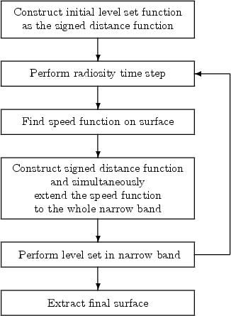
Figure 5.7 shows an overview of the simulation flow achieved
when using TOPO3D. The simulation begins at the WSS. WSS provides
us with the initial surface which is then propagated. The initial surface is
represented by a set of triangles. In the next step the level set
function is initialized with the signed distance function. After this
step the time stepping is started. At each time step a data exchange
between the simulation model and the level set kernel takes place. The
simulation model provides the speed function needed by the level set kernel
to propagate the surface. Vice versa the model also needs
information about the actual distance function from the surface
propagation step. After ![]() time steps the final surface is extracted
as the zero level set of the level set function. After coarsening the
final surface and merging it with the initial surface, a meshing
step is performed and the information is stored in WSS.
time steps the final surface is extracted
as the zero level set of the level set function. After coarsening the
final surface and merging it with the initial surface, a meshing
step is performed and the information is stored in WSS.
To advance the level set function we have used a second order space
convex finite difference
scheme [24,20,19,13].
Consider ![]() ,
, ![]() ,
,
![]() , and
, and ![]() as discretization steps in space and
time, respectively. As mentioned in Section 5.6, a necessary
condition for the stability of this scheme is the
CFL condition which requires that
as discretization steps in space and
time, respectively. As mentioned in Section 5.6, a necessary
condition for the stability of this scheme is the
CFL condition which requires that
However, there is a problem stemming from the CFL condition, which
limits the simulator performance. If we increase the spatial
resolution by ![]() , assuming that
, assuming that ![]() remains
constant, we have to reduce the maximum
remains
constant, we have to reduce the maximum ![]() by the same factor
by the same factor
![]() , which increases the number of simulation steps by
, which increases the number of simulation steps by ![]() to
reach the same thickness. Furthermore, an increase in spatial
resolution by
to
reach the same thickness. Furthermore, an increase in spatial
resolution by ![]() approximately increases the number of
extracted surface elements by
approximately increases the number of
extracted surface elements by
![]() in three
dimensions. Therefore, the computational
effort of the visibility determination is increased by
in three
dimensions. Therefore, the computational
effort of the visibility determination is increased by
![]() . In total, an
increase in spatial resolution by
. In total, an
increase in spatial resolution by ![]() leads to a minimal increase of
simulation time by a factor
leads to a minimal increase of
simulation time by a factor
![]() , if the most
precise visibility calculation is used.
, if the most
precise visibility calculation is used.
![\includegraphics[width=\linewidth]{IllustrationOfVisibility2.eps}](img246.png)

![\includegraphics[width=\linewidth]{figures/main_diagram}](img346.png)