Subsections

• 4.1 The Models
  • 4.1.1 Line Source Model
  • 4.1.2 Flux Dependent Sticking Coefficient Model
  • 4.1.3 Two Species Model
  
  
• 4.2 Summary

4. Simulation Models for Deposition of Silicon Dioxide Layers from TEOS

During the fabrication of an IC a wafer has to undergo many processes. Each process accomplishes a specific change in the state of the wafer. Some of these processes can be described using relatively simple models. However, many processes require more complex models to be described reliably. Process modeling and simulations have been used to provide a general understanding and not for quantitative prediction of processes [18,17]. Therefore, for more general prediction and analysis, a general topography simulator must use detailed descriptions of chemical reactions with chemical reaction rates and thermodynamic properties of the species obtained by experiment and/or by calculation. In addition, topography simulations should be done in conjunction with reactor-scale simulations in order to compute gas transport to and from the reactive surface in a self-consistent manner.

One standard way to accurately perform a feature-scale simulation of CVD processes is to use a system of reversible elementary chemical reactions which are implemented in the general topography simulator using CHEMKIN or SURFACE CHEMKIN [49,26].

In order to quantitatively understand and optimize the reaction conditions in a CVD or plasma process, complex chemical reaction flows have to be simulated. Although reaction conditions and geometries are very variable among the applications of chemically reaction flows, all of them need accurate and detailed descriptions of the chemical kinetics occurring in the gas-phase or on reactive surfaces. Chemical reaction mechanisms containing hundreds of reactions and involving fifty or more chemical species are not uncommon in such models. The CHEMKIN suite of codes broadly consists of three packages for dealing with gas-phase reaction kinetics, heterogeneous reaction kinetics, and species transport properties [50].

The CHEMKIN software package has been developed for incorporating the complex mechanisms of gas phase chemical reactions into numerical simulations [49]. Thereafter, different codes based on CHEMKIN have been implemented that solve chemical reacting flows. In order to easily enable the user to specify the necessary input information, the CHEMKIN interface uses a high-level symbolic interpreter. This interpreter parses the information and passes it to a CHEMKIN application code. The user writes an input file declaring the chemical elements in the problem, the name of each chemical species, thermochemical information about each chemical species, the rate constant information, and a list of chemical reactions which is written in the same manner that a chemist would write them, i.e., a list of reactants converted to products [50]. The thermochemical information is entered as a series of polynomial coefficients describing the species entropy, enthalpy, and heat capacity as a function of temperature. Because the information about the reaction mechanisms is parsed and summarized by the CHEMKIN interpreter, if the user desires to modify the reaction mechanisms by adding species or deleting a reaction, for instance, only the interpreter input file has to be changed, while the CHEMKIN application code (for example, a rotating-disk reactor simulation code) does not have to be altered. The modular approach of separating the description of the chemistry from the set-up and solution of the reacting flow problem gives the software designer great flexibility in writing chemical-mechanism-independent code. In addition, the same mechanism can be used in different chemically reacting flow codes without changes.

The SURFACE CHEMKIN package has been developed for specifying the mechanistic and kinetic rates of heterogeneous chemical reactions[50]. SURFACE CHEMKIN is run in connection with CHEMKIN and the execution of the CHEMKIN interpreter is required before the SURFACE CHEMKIN interpreter can be run. The user interface for SURFACE CHEMKIN is very similar to that of CHEMKIN, but is extended to account for the richer nomenclature and formalism required to specify heterogeneous reaction mechanisms.

The transport software package provides the gas-phase transport properties. It also includes the effects of such phenomena as thermal diffusion and provides the calculation of the pure species viscosity, pure species thermal conductivity, and binary diffusion coefficients for every gas-phase species in the mechanism, as a function of the temperature.

A number of high-level CHEMKIN applications for chemically reacting flow simulation has been produced during the last years. Many researchers around the world are using these codes and while the challenge for the researcher at the beginning was the software development, this is nowadays developing a realistic reaction mechanism for an accurate description of the system of interest.

These software packages have to describe chemical kinetic reactions in a reactor and on the surface. They consist of a thermodynamic database, interpreters to transform user-defined, human-readable chemical reaction mechanisms into rate equations suitable for numerical calculation, and subroutine libraries to perform kinetics calculation within simulation codes. The link between CHEMKIN and a topography simulator has two major implications. First, a wide range of chemical reaction systems already expressed in the CHEMKIN formalism can be simulated immediately both at the reactor-scale, using several CHEMKIN-based reactor simulation codes, and at the feature-scale, using a topography simulator, without manual reinterpretation of the reactions into a different reaction format.

This allows feature-scale simulators to employ detailed reaction mechanisms previously developed for the reactor-scale. Second, computational analysis of processes can be made at one scale with immediate feedback to the other scales. For instance, a predicted film profile inside a submicron feature will not only be sensitive to transport in the reactor and in the submicron feature, but also to the choice of reaction mechanisms. Therefore, the individual models at different length scales must be coupled by feeding the results from higher order scales into the lower order scales and feeding back the lower orders to the higher order scales for forming a tightly coupled solution.

However, the basic difficulty of combining reactor- and feature-scale simulations has been the inherent disparity in length scales. These length scales can span more than six orders of magnitude, i.e., from about a meter at the reactor-scale to submicrometer at the feature-scale. Cale et al. [17] investigated a different approach which consists of using a reactor-scale simulator to predict the conditions near the wafer surface based on the operating conditions. These local conditions are then used in a feature-scale simulator to predict deposition profiles at different positions on the wafer surface. Holleman et al. [17] have attempted to determine the effect of feature-scale on the reactor-scale, of course, with only focussing on the feature-scale. Thus, in both of the above approaches, there was no feedback of information of one scale to the other one.

Another approach used to link up reactor- and feature-scale simulations is the effective reactivity function formulation described by Rogers and Jensen [17]. In this approach the reactor- and feature-scale simulations are linked together using an effective reactivity $\varepsilon$, which includes effects of both surface variations as well as feature-scale transport. A Monte Carlo-based ballistic transport (cf. Section 4.1) scheme is used to calculate the effective reactivity of a single feature. The reactivity of each set of features is then linearly superimposed to obtain $\varepsilon$. To resolve the gradients in $\varepsilon$ one has to guarantee that the source plane for the Monte Carlo simulation is at a sufficient distance from the wafer surface. Satisfying this requirement is an elementary step to use superimposition.

The effective reactivity is then fed into the reactor-scale simulation as an enhancement factor to the flux boundary condition over a blanket area. The reactor- and feature-scale simulations are then iterated to arrive at a consistent solution. This technique has been applied to the simulation of tungsten deposition. While this technique can be used to couple reactor- and feature-scale simulations, the prohibitive time requirements for each feature-scale simulation and calculation of $\varepsilon$, and the iterative nature of this process, make it difficult to efficiently use this approach.

The above mentioned two-scale approaches assume that the reactor-scale simulator, utilizing a mesh which is much coarser than typical for a feature-scale simulation, can compute appropriate conditions for a particular feature. Furthermore, the structure of the wafer surface representation in the two-scale approach is necessarily crude [30]. When using a feature-scale simulator at a particular boundary of the reactor-scale, the implicit assumption is that any single feature is a part of a cluster of identical features for which the single feature is a representative member. But in order to represent such a cluster appropriately in a numerical sense, several grid points across the cluster are needed. This limits the reactor-scale simulator to model unrealistically large feature clusters. However, the details of the surface structure of a realistic die with several much smaller clusters can not be represented. Thus, feedback from the feature-scale to the reactor-scale is indeed difficult.

Gobbert et al. [30] introduced a mesoscopic-scale model to simulate deposition processes at the scale of a few dies. It was used to provide an understanding of the deposition processes at a scale inaccessible by both reactor- and feature-scale models. This approach not only avoids the excessive grid resolution that is necessary for a single model, but also allows to capture the underlying physics by varying the model description according to the scale. The model regime changes from continuum transport (cf. Section 4.1) to ballistic transport at different length scales. This implemented model involves a transient reactor-scale simulator for continuum mechanics, which solves the governing equations of mass, momentum, heat, and species concentrations as a function of position and time. On the reactor-scale, the wafer topography is not explicitly taken into account, and the information from the other scales is only incorporated as a net flux boundary condition on all nodes of the final grids representing the wafer. At the next level which corresponds to the meso-scale, continuum equations are still valid and the same solver is used as for the reactor-scale problem. However, at the feature-scale the continuum equations are no longer valid and the transport of individual molecules has to be taken into account to accurately represent the underlying physics.

This three-scale simulation approach couples numerical meshes whose typical mesh sizes are separated by fewer orders of magnitude than in the two-scale approach. Moreover, due to meaningful feedback from the smaller scales to the larger ones, reactor scale simulations may account for the depletion or accumulation of chemicals close to the surface [30]. However, it is important to note that even in the coarsest implementation of the mesoscopic model, which assumes all features inside one cluster to be identical, there can be variations from one cluster to the others both in geometry and in reactor conditions. Indeed, an implementation using a sufficient number of mesh points can even represent variations inside a cluster. Furthermore, this model has also limited predictive capability because of its dependence on input parameters from the two other scales. A truly predictive simulator must have the capability to couple phenomena occurring at the reactor-scale, meso-scale, as well as the feature-scale, where information from each scale is transferred correctly and coupled tightly to the other scales.

Generally, the proposed models for the deposition of SiO$_2$ from TEOS CVD process fall into two categories: first as mentioned above, those which use complex surface reaction models including the integration of reactor-, meso-, and feature-scale. Second, those which use the sticking coefficient model with one or more species.

In spite of the complexity of the models from the first category, their quantitative predictability is still very limited for processes of industrial interest. Therefore, the simpler calibrated sticking coefficient models provide good alternatives for process investigations and especially for time-consuming optimizations and inverse modeling tasks. The parameters of simulation are evaluated and optimized using SIESTA (simulation environment for semiconductor technology analysis)[16,35].

The goal of this chapter is to identify simulation models for the deposition of silicon dioxide layers from TEOS in a CVD process and to calibrate the parameters of these models by comparing simulation results to SEM images of deposited layers in trenches with widely different aspect ratios. We describe the models which lead to the best results. We also draw conclusions regarding the usefulness of the models.

4.1 The Models

A transport model can be characterized by the ratio of the mean free path length of the species to the characteristic length scale (the largest dimension of the feature). This ratio is called $K_{n}$ (Knudsen number) [18]. A high $K_{n}$ ($\gg1$) implies that the frequency of particle-particle collisions is negligible relative to particle-surface collisions, i.e., the process is in free molecular regime or BTRM (ballistic transport and reaction model). A small $K_{n}$ ($\ll1$) implies that collisions between particles occur much more frequently than collisions between particles and the feature surface. This is called continuum transport regime. A $K_{n}$ about one implies the transition regime where the order of magnitude of the particle-particle and particle-surface collisions are approximately the same [18].

Because of the low pressure condition of the TEOS process, the mean free path length of the species is much higher than the feature dimensions and thus $K_{n}$ is $\gg1$. The process is in the free molecular regime and the radiosity model can be applied for the transport of the particles [80].

In the earliest attempts at our institute [37], a single trench was simulated successfully. The so called point-shape source model was used, where the source of species is assumed to be a single point or a very small number of points in the middle of the simulation domain or along a line above the trench. The flux distribution around the vertical axis follows a cosine form (this distribution is also assumed for the models presented in the next sections) and the direct flux received at the surface elements was assumed to be proportional to the inverse of the distance between the source and the middle point of a surface element. However, the optimum sticking factors showed a strong dependence on the aspect ratio [37].

Figure 4.1: Illustration of the calculation of the incoming flux.

4.1.1 Line Source Model

As mentioned above, the previous model is not able to predictively simulate a set of trenches with widely different aspect ratios. There are additional problems as the model does not allow to simulate several trenches back to back (cf. Chapter 6). The first idea for overcoming this problem was to set many point-shaped sources along a source line above the wafer. However, one open question is at which distances the points must be placed, i.e., how many source points and how far do we have to extend the source line beyond the simulation domain to obtain a reliable number of sources? To avoid the problem of asymmetry which becomes apparent with this solution, if one half of the trench sees a source point more than the other half due to the discretization, the number of points has to be increased above a certain threshold value which is related to the chosen discretization. However, the simulation time is increased considerably, because the number of visibility tests between the surface elements and point-shaped sources increases significantly. The line source model presented in the following is a good alternative to overcome the mentioned problems.

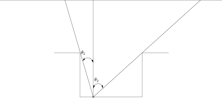
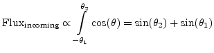
In this model [9] the source consists of a line of continuous point-shaped sources above the trench as shown in Figure 4.1. Using this model, one of the expensive time consuming parts of the discrete set of point-shaped sources, namely, the visibility test is moderated and the computation time is therefore significantly reduced. In our experience, visibility tests in steps of one degree give sufficient accuracy. Therefore, instead of separate visibility tests among a surface element and different sources, a complete visibility test is performed in a maximum 180 steps, which is the case if a surface segment is on the flat open part of the trench. After the calculation of the visibility angle between a surface element and the source line the incoming flux can be calculated. In this model the incoming flux has been assumed to depend only on the visibility angle between the surface elements and the source line as follows:

$$\mathrm{Flux_{incoming}}\propto \int \limits_{-\theta_{1}}^{\theta_{2}}\cos(\theta)=\sin(\theta_{2})+\sin(\theta_{1})$$

Two different sticking coefficients have been identified by calibration using SIESTA. The first coefficient denotes the sticking probability of the particles arriving directly from the source on the surface while the second coefficient describes the reflection probability of the particles from the surface elements. Although the outline of the trench for a low aspect ratio is reproduced predictively as shown in Figure 4.2, it is difficult to reproduce both the upper and lower part of the trenches at the same time for a higher aspect ratio as demonstrated in Figure 4.3.

4.1.2 Flux Dependent Sticking Coefficient Model

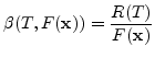
Although in the previous model the sticking coefficients have been assumed to be constant, the overall sticking coefficient for a species can be written as a function of the local fluxes of the reacting species on the surface [19]. Assuming that the deposition from TEOS is through heterogeneous decomposition of species with the rate depending on temperature and the flux of the species [19] the overall sticking coefficient can be written as

$$\beta(T,F({\mathbf{x}}))=\frac{R(T)}{F({\mathbf{x}})}$$ (4.1)

where $R$ is the number of molecules per area and per time that become part of the film, and $F(\mathbf{x})$ denotes the position-dependent flux. If the heterogeneous deposition reaction follows $m$th order kinetics with respect to Arrhenius temperature dependence of the rate parameter $k(T)$, then

Figure 4.2: Comparison of simulation and measurement for the continuous line source model for a trench with a low aspect ratio.

Figure 4.3: Comparison of simulation and measurement for the continuous line source model for a trench with a higher aspect ratio.

$$R(T)=k_{0}\mathrm{exp}(\frac{-E_{a}}{k_{B}T})F(\mathbf{x})^{m}=k(T)F(\mathbf{x})^{m}$$ (4.2)

where $k_{0}$ is the temperature independent pre-exponential factor and $E_{a}$ is the activation energy for the reaction. (4.2) is a commonly used form for heterogeneous kinetic expressions which are usually determined by analyzing film growth rates on a flat substrate as a function of temperature and reactant concentrations. Substituting (4.2) into (4.1) results in

$$\beta(T,F({\mathbf{x}}))=k(T)F({\mathbf{x}})^{m-1}.$$ (4.3)

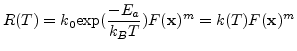
Based on (4.3) and two further assumptions we developed a flux dependent sticking coefficient model [9]. The first assumption is that the temperature $T$ remains constant and the second is that the deposition of silicon dioxide from TEOS follows a half order reaction [19], i.e., $m=1/2$. Therefore, the sticking coefficient is $\beta=\beta_0 F({\mathbf{x}})^{-1/2}$, where $\beta_0$ is a constant scaling factor to guarantee that sticking coefficients are always equal to or less than one.

The simulation results are in good agreement with the measurements for trenches with low aspect ratio as shown in Figure 4.4. For higher aspect ratios, however, the amount of material deposited on the side-walls is overestimated as shown in Figure 4.5. This may result in spurious void formations.

4.1.3 Two Species Model

With the last two models we have reached the limits of models which assume a single species for the deposition of silicon dioxide from TEOS.

Generally there are two approaches to model the kinetics which control a LPCVD (low pressure CVD) process: surface kinetics dominated and transport dominated.

The surface kinetics dominated model has been pursued by many authors modeling deposition on flat surfaces [24,55,21]. Here, it is assumed that the source gases do not react until they reach the wafer surface and thus, the deposition is totally controlled by surface reactions. In this case, modeling proceeds by assuming different surface reaction paths, and comparing the resulting rate kinetics with the observed dependence of the growth rate on partial pressures calculated from the source gas flow rates. It is assumed that the reaction path model whose kinetics best matches the measurements is the correct model. While this approach has been successful for some deposition processes, it leads to models with too many parameters for topography simulations. In addition, the assumption that no pre-reaction takes place does not hold well when deposition shows poor conformality. Therefore, one has to assume a highly reactive species whose deposition rate is inconsistent with the source species concentrations [48].

Figure 4.4: Comparison of simulation and measurement for the flux dependent sticking coefficient model for a trench with a low aspect ratio.

Figure 4.5: Comparison of simulation and measurement for the flux dependent sticking coefficient model for a trench with a higher aspect ratio.

With the second approach, as described in [48], the deposition is assumed to be controlled by the transport inside the device structure of one or two rate limiting species which contribute considerably for determining the growth rate. These species are not confined to the source gas species, but could be the result of gas phase reactions or reactions on surfaces of the reactor. The model does not deal with the details of the chemistry of growth, which is not completely understood in the case of deposition of silicon dioxide from TEOS. However, this model can be extended easily to take detailed growth chemistry into account if these details are known.

The incident species is adsorbed at the surface and depending on the reaction probability (reactive sticking coefficient) of the species with the surface, the incident species may be re-emitted from the surface, react at the point of incidence and become a part of the surface or diffuse along the surface to another surface site and then react or be re-emitted.

Studies have shown [12,56,48] that for LPCVD of silicon dioxide from TEOS, re-emission instead of surface diffusion is the most likely surface-species interaction mechanism. Therefore, we also neglect surface diffusion and only consider re-emission in our simulations.

An often debated issue related to the single sticking coefficient model for the LPCVD of silicon dioxide from TEOS is the mechanism which has been commonly suggested. This mechanism assumes that silicon dioxide is deposited by TEOS decomposition at the surface. However, this does not describe the formation of intermediate reaction products in the gas phase or on the surface. It has been proposed in [48] that there may be a second reaction path in the LPCVD of silicon dioxide from TEOS. This leads to formation of a very reactive intermediate, due to gas phase reactions, which reacts with the surface to form silicon dioxide. The reactions used there, are merely a suggestion of one possible set of reactions but do not rule out any other reaction paths. The model considers two species but does not care how they are formed. Therefore, the model is independent of the reaction path for the formation of the species.

Based on the idea of this model we have developed our two species model [9], which not only considers the transport of a single gas species above the wafer and its sticking and reflection on the surface, but also producing a second species at the surface because of the chemical reaction happening in interaction between the first species and the surface. We assumed that the flux of the second species is proportional to the flux of the species coming directly from the source. In our model there are two possibilities to include the effects of the second species, either to consider increasing or decreasing the deposition rate.

The following equation has been used for the calculation of the total flux on the surface segments

$$F_{{\mathrm{total}}}= F_{{\mathrm{A}}}\cdot(1\pm \alpha F_{{\mathrm{B}}})$$ (4.4)

where $F_{{\mathrm{total}}}$ is the total flux at the surface segment, $F_{{\mathrm{A}}}$ is the flux of the first species, $\alpha$ is a proportional factor, and $F_{{\mathrm{B}}}$ is a normed flux of the second species. It is important to note that $F_{{\mathrm{A}}}$ and $F_{{\mathrm{B}}}$ in this model and the flux in Section 4.1.2 can be calculated using an iterative solver. This iterative solver can be set to stop the calculation if the difference between the flux value at the new step and the last step is smaller than a user defined error term (cf. Section 5.10). This model shows excellent agreement with SEM images as shown in Figure 4.6 and Figure 4.7.

4.2 Summary

A multitude of deposition models for TEOS processes as well as means for the calibration of simulation results to measurements have been proposed. In summary we find that a two-species model yields the best results among the three different deposition models investigated, both for high and low aspect ratio trenches. More complex deposition models can be avoided with this model.

Figure 4.6: Comparison of simulation and measurement for the two species model for a trench with a low aspect ratio.

Figure 4.7: Comparison of simulation and measurement for the two species model for a trench with a higher aspect ratio.