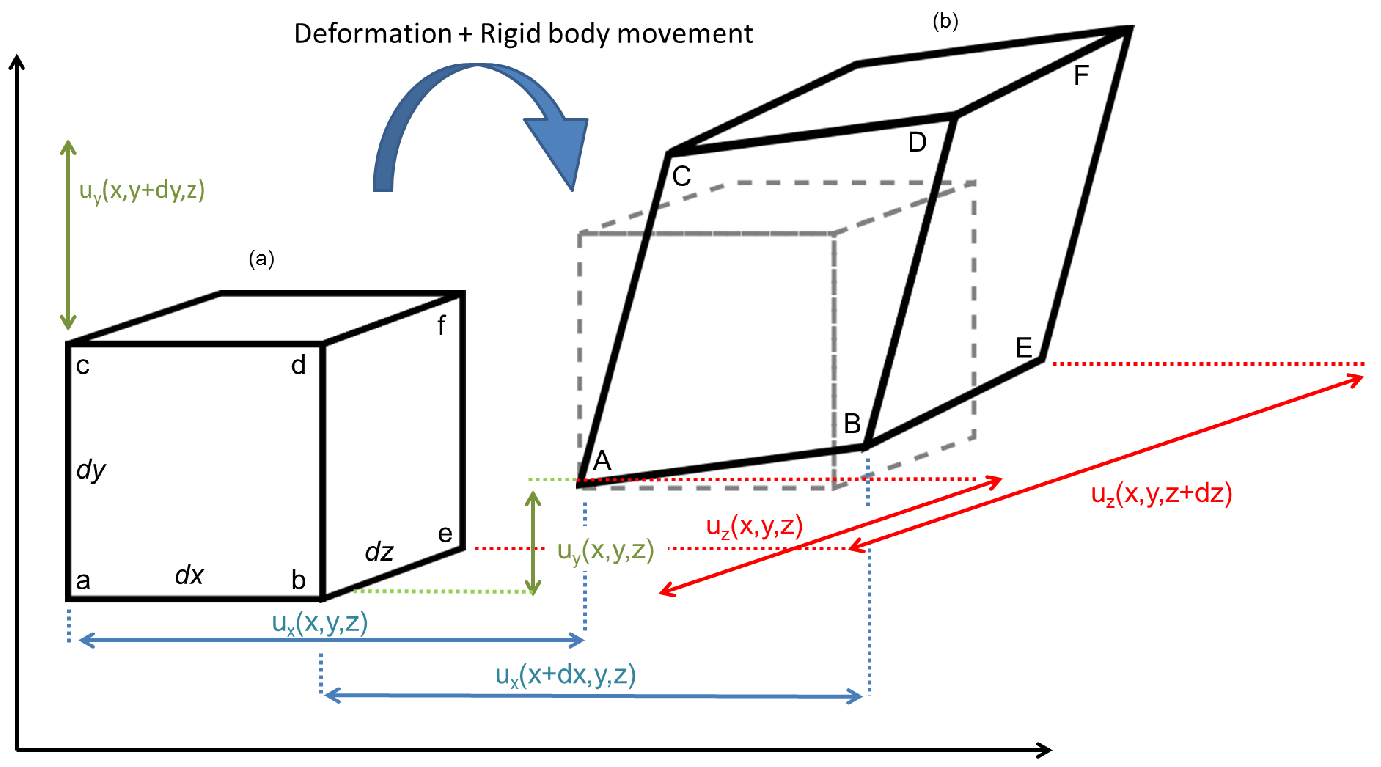
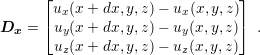
| Figure 2.2.: | General deformation of a body after external loading. Rigid body movements such as translation and rotation are included, although they should not count for the final body deformed state. |
Infinitesimal strain theory describes solid behavior for deformations much smaller than the body dimensions [37][39]. Qualitatively, this means that the body geometry is assumed unchanged during the deformation process. It can sound inconsistent, but it is the most common situation for solids. For example, when a car drives over a bridge, it certainly applies some force on the bridge and such force leads to some deformation. However, one can say that the bridge remains immutable, since any deformation is irrelevant, when the full enormity of the bridge is considered. For an engineer it is still important to know the effect which the car has on the bridge. For that analysis, the infinitesimal strain theory is applied.
There are two different ways to describe very small deformations of solids. The first one is based on the linearization of Lagrangian or Eulerian strain tensors of finite strain theory [40], a generalization of infinite strain theory. The second method is a geometric based description, which is derived in the section which follows.
Consider the infinitesimal volume of a solid as in Fig. 2.2a. Due to some external influence (e.g. force, heat) this infinitesimal body is deformed, assuming the shape of the Fig. 2.2b. Deformation can be quantified as the amount of elongation, contraction or torsion an infinitesimal side suffers.
| Figure 2.2.: | General deformation of a body after external loading. Rigid body movements such as translation and rotation are included, although they should not count for the final body deformed state. |
The displacement field accounts for every movement inside the solid, therefore rigid body
translation and rotation are included. To measure the deformation of a body, the side ab can
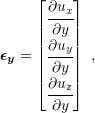
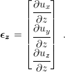
be taken into consideration. The deformation of the side ab ( ) is given by
the difference between the displacement vectors (
) is given by
the difference between the displacement vectors ( ) of the points b and
a
) of the points b and
a
 | (2.1) |
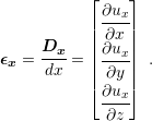
The vector  can be explicitly defined in terms of each of its components
 | (2.2) |
The first term of each component can be expanded in Taylor series as shown in (2.3). Only
the term for  is shown for the sake of brevity:
 | (2.3) |
Since very small deformations are considered, any term of the second order can be ignored
and the vector  is rewritten as in
 | (2.4) |
The vector  specifies the extent of the deformation of the side ab in the direction of the
three coordinate axis. However, it is more convenient to express the deformation in
normalized units related to the original ab size (dx) as in
specifies the extent of the deformation of the side ab in the direction of the
three coordinate axis. However, it is more convenient to express the deformation in
normalized units related to the original ab size (dx) as in
 | (2.5) |
This relative measure of deformation is known as strain. This definition provides a better
feeling of how much the solid has changed in comparison to the undeformed solid. The
strain in the original direction of the side ab (x-direction) is called normal strain ( ).
It reflects the tendency of the points, originally aligned (in this case, parallel to x-axis), to
move away (stretch) or to approach (contract) each other along the same direction of the
side ab. The deformation of the other two components of
).
It reflects the tendency of the points, originally aligned (in this case, parallel to x-axis), to
move away (stretch) or to approach (contract) each other along the same direction of the
side ab. The deformation of the other two components of  describes the tendency of the
points to skew in relation to each other toward the direction of each component (y or z).
The same procedure can be repeated for each side (cd and ef ) parallel to the
coordinate axis of the infinitesimal solid. The same result holds, except for an index
change.
describes the tendency of the
points to skew in relation to each other toward the direction of each component (y or z).
The same procedure can be repeated for each side (cd and ef ) parallel to the
coordinate axis of the infinitesimal solid. The same result holds, except for an index
change.
 | (2.6) |
 | (2.7) |
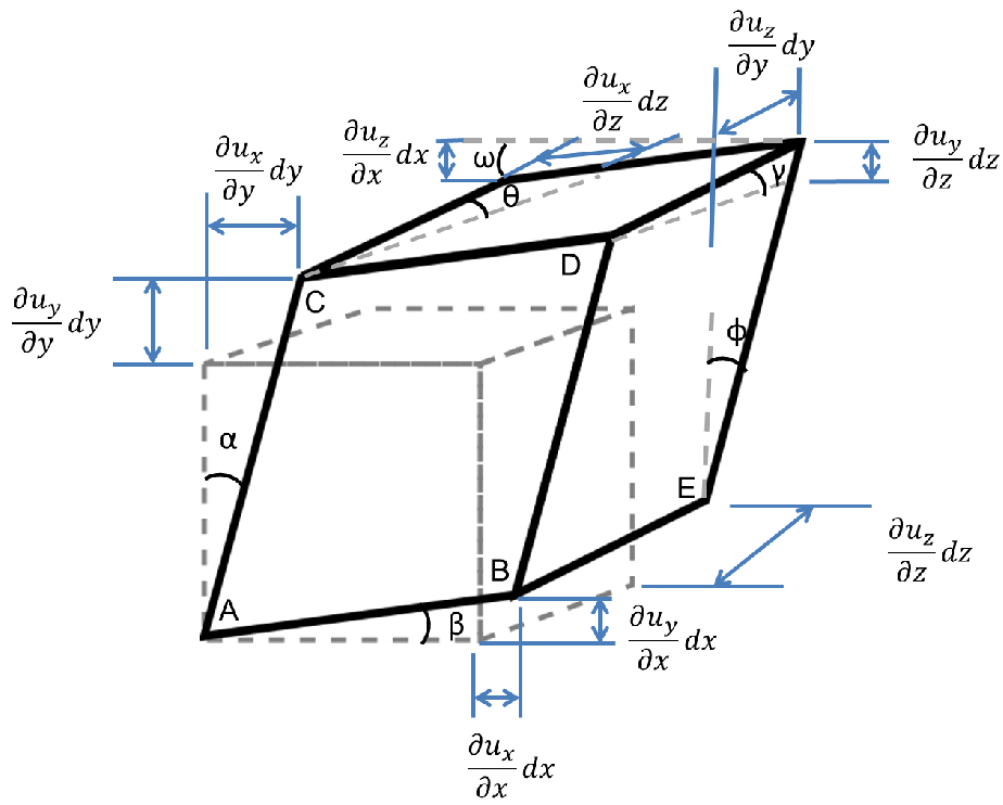
The skew deformations are related to the angles formed between the original sides
and the deformed sides as defined in Fig. 2.3 ( ,
,  ,
,  ,
,  ,
,  , and
, and  ). For
example, the angle
). For
example, the angle  can be expressed in terms of the skew y-component according
to
can be expressed in terms of the skew y-component according
to
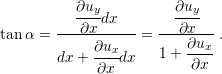 | (2.8) |
Where, for  the relation (2.8) can be further simplified by
 | (2.9) |
A similar relation also holds for  regarding the skew x-component.
A common method to measure the skew of a solid is to sum up the angular deviation in a
particular coordinate plane. For example the skew of the solid in the plane-xy is given by
the sum of  and
and  . For the plane-xz is the sum of
  and
and  , and for the plane-yz is the
sum of
, and for the plane-yz is the
sum of  and
and  . This measure is called shear strain.
In summary, a solid deformation is represented by 3 normal strain components (one for each direction) and 3 shear strain components (one for each coordinate plane). The usual nomenclature is stated below and the geometrical view of the strained component is sketched in Fig. 2.3.
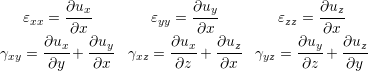 | (2.10) |
For mathematical handling, it is very convenient to represent the strains of a solid deformation as a tensor:
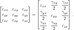 | (2.11) |
The factor  is added in order to simplify the manipulation of constants in future
applications of the strain tensor. The strain tensor is symmetric and has 3 components not
discussed previously, namely
is added in order to simplify the manipulation of constants in future
applications of the strain tensor. The strain tensor is symmetric and has 3 components not
discussed previously, namely  ,
,  , and
, and  , where
  ,
,  , and
, and
 . Those components represent the complement of the skew angles in each
coordinate plane, as depicted in Fig. 2.4.
. Those components represent the complement of the skew angles in each
coordinate plane, as depicted in Fig. 2.4.
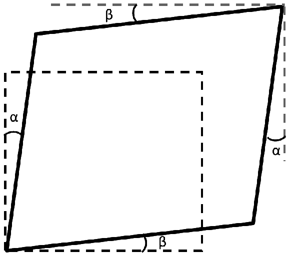
| Figure 2.4.: | Complementary angles in the plane xy. The indicated angles on the bottom left corner of the quadrilateral are equal to those on the upper right corner, due to triangle symmetry. |
Every solid body reacts to deformations. Internal forces arise in the solid as a response to strain, similar to the restoration force in a spring. These forces are known as stress and act to restore the undeformed state of the body [39]. Stress might have several sources: it can be a reaction to external forces, temperature variation, or electromagnetic fields (e.g. piezoelectric devices). Stress can also arise during material fabrication, due to microstructural phenomena. Those are referred to as residual stress or intrinsic stress. An example is the formation of metal lines for semiconductor devices. The characteristics of the metal growth process and the particular interaction between the metal and silicon create residual stress in the lines. The same situation occurs in oxide growth, material deposition, and any other process which involves the introduction of new materials during thin films fabrication.
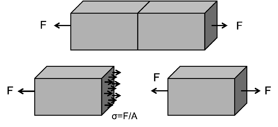
The stress is defined qualitatively as the force between adjacent parts of a solid acting on an imaginary surface, divided by the area of this surface, as sketched in Fig. 2.5. The force’s magnitude and direction usually depend on the chosen surface. The situation depicted in Fig. 2.6 is used as an example.
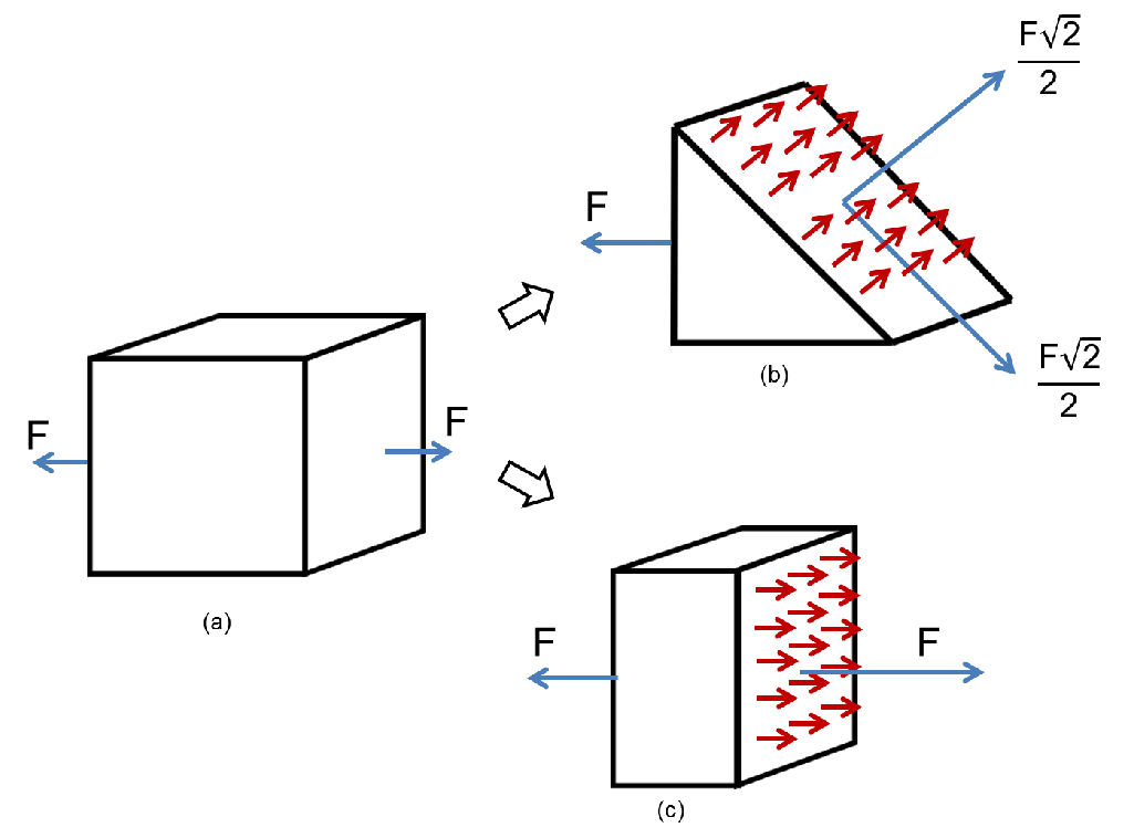
| Figure 2.6.: | The dependence of stress on the chosen plane. A body under a load (a) can have different stress configurations at a point, depending on the considered plane (b and c). However, they must describe the same physical phenomenon. |
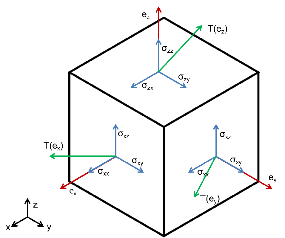
According to the chosen imaginary plane, the force applied on it will be such as to satisfy the force equilibrium condition of the solid. Therefore a proper description of the stress at a point of a body cannot be accomplished by a single vector and the information about the chosen plane should be included. Augustin-Louis Cauchy realized that the force has a linear relationship with the surface normal [39][40]. He described this relationship as tensor which is independent of the chosen surface and describes only the stress state at a specific point in a body, as defined in
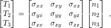 | (2.12) |
where  is the force vector on the surface with normal
  and
and  is the stress tensor
suggested by Cauchy. Additionally, Cauchy has shown that the stress tensor at a point P is
formed by the stress vectors of 3 mutually perpendicular planes which pass through P [41].
The stress vector in any other plane passing through P can be obtained by a coordinate
transformation of the stress tensor. Fig. 2.7 depicts Cauchy stress definition in a
cube.
is the stress tensor
suggested by Cauchy. Additionally, Cauchy has shown that the stress tensor at a point P is
formed by the stress vectors of 3 mutually perpendicular planes which pass through P [41].
The stress vector in any other plane passing through P can be obtained by a coordinate
transformation of the stress tensor. Fig. 2.7 depicts Cauchy stress definition in a
cube.
Like the strain nomenclature, the stress components have special names according to their direction. The components aligned to the normal of the three perpendicular planes are called normal stress and those perpendicular to the normal of the plane are the shear stress. The Cartesian coordinate system is suitable for the application of Cauchy’s definition. The sub-indexes used in (2.12) refer to the Cartesian coordinate system (But any other coordinate system can be used without (2.12) losing its generality).
An important stress tensor’s property is symmetry. The stress must hold this property, in order to satisfy conservation of angular momentum. Since the stress tensor is a second-order object (matrix), the symmetry eases the mathematical handling of the tensor. It is possible to prove that a symmetric matrix has real eigenvalues and perpendicular eigenvectors [42]. Hence, the eigenvectors can define a space to apply the Cauchy stress definition. Furthermore, in this space the stress tensor is a diagonal matrix of the eigenvalues. This means that, in the “eigenspace” the stress tensor has no shear stress, it has only normal stress. These components (eigenvalues) are called principal stresses and the eigenvectors are known as the principal stress directions.