
The elastic behavior of solids can be modeled by the same principle which governs spring deformations, known as Hooke’s law. The law suggests a linear relationship between the deformation and the force applied to a string or in a solid. Hence, the relation stress-strain in solid bodies in the elastic regime can be expressed by
|
| (2.13) |
where  is a linear mapping between the two tensors
  and
and  . This implies
that
. This implies
that  is a fourth-order tensor with 81 components (each of the 9 strain tensor
components is related with each of the 9 stress tensor components). However,
due to the symmetry of the strain and stress tensors the number of independent
components of
is a fourth-order tensor with 81 components (each of the 9 strain tensor
components is related with each of the 9 stress tensor components). However,
due to the symmetry of the strain and stress tensors the number of independent
components of  can be reduced to 21. This simplification process can be seen
graphically in Fig. 2.8. Therefore a 6x6 symmetric matrix is a convenient way
for representing the tensor
can be reduced to 21. This simplification process can be seen
graphically in Fig. 2.8. Therefore a 6x6 symmetric matrix is a convenient way
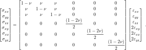
for representing the tensor  and the stress-strain relation can be rewritten as
in
and the stress-strain relation can be rewritten as
in
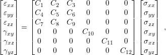 | (2.14) |
where  are constants to be determined in the next sections. The matrix in (2.14) is also
known as stiffness matrix.
are constants to be determined in the next sections. The matrix in (2.14) is also
known as stiffness matrix.
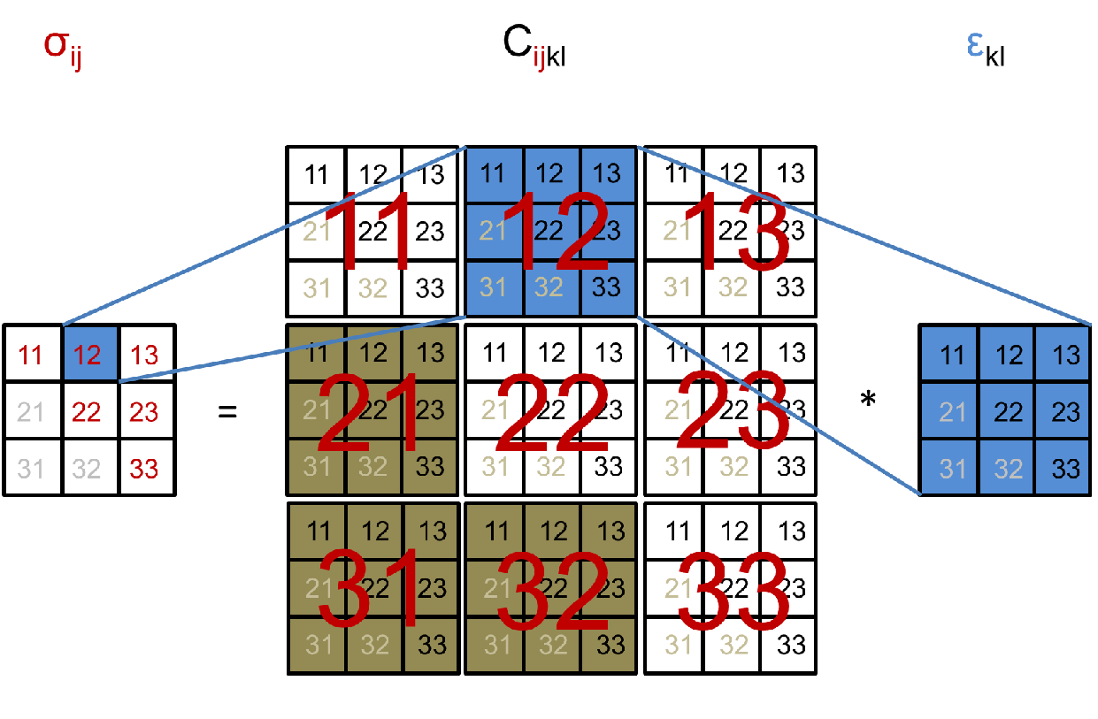
| Figure 2.8.: | Visualization of the tensorial Hooke’s law. Strain symmetry forces
symmetry on the  tensor on all components in the form tensor on all components in the form  , ,  , and , and  indicated by numbers in gray. Strain symmetry is enforced on the components
  , ,
 , and , and  indicated by the brown squares. indicated by the brown squares. |
The coefficients of the stiffness matrix for the normal components can be obtained from the superposition of two effects in a solid. For doing so, a force which is applied to a body is considered, as depicted in Fig. 2.9.
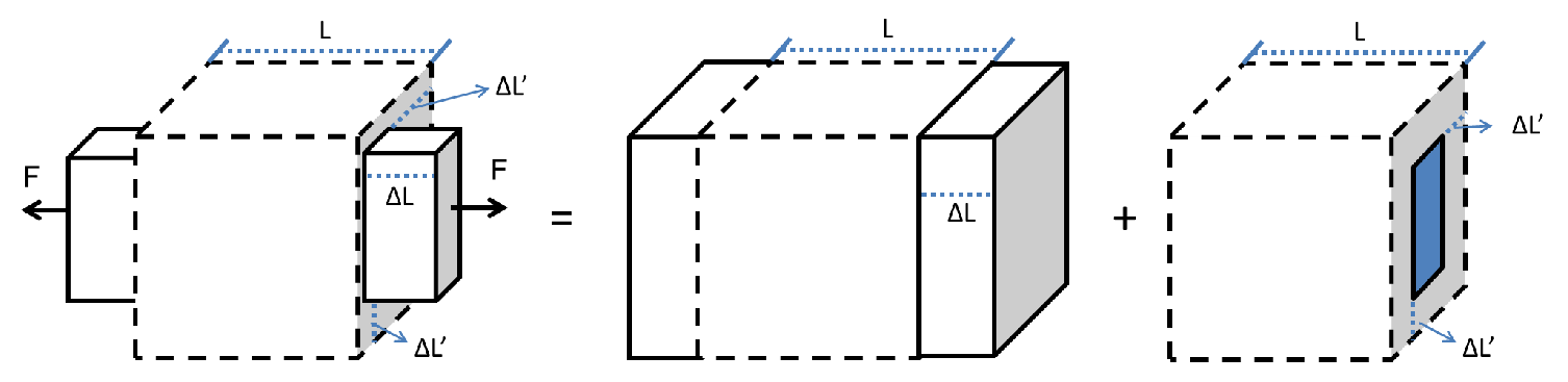
| Figure 2.9.: | Superposition of effects during an uniaxial loading of a body, where
 is the normal strain is the normal strain  along the direction of the applied force and along the direction of the applied force and
 is the normal strain is the normal strain  in the directions perpendicular to the force. in the directions perpendicular to the force. |
The body stretches in the same direction of the load and shrinks in the perpendicular direction. These two deformations can be treated separately and then added together by the principle of linear superposition of the resulting strains produced by each phenomena depicted in Fig. 2.9. The strain in the parallel direction is given by the uniaxial (1D) Hooke’s Law. Consequently, the linear mapping between the stress and strain is described by a constant
 | (2.15) |
where,  is the strain in the direction to the parallel to the applied force. It should
be noted that in the one-dimensional case the stress and the strain are no longer a tensor
but a scalar. The proportionality constant E is known as Young modulus (or elastic
modulus). The Young’s modulus depends on the material of the solid and characterizes the
material stiffness. Materials with high values of E are stiffer and harder to deform. Typical
values of Young’s modulus for different materials essential in semiconductor industry are
listed in Table 2.1.
is the strain in the direction to the parallel to the applied force. It should
be noted that in the one-dimensional case the stress and the strain are no longer a tensor
but a scalar. The proportionality constant E is known as Young modulus (or elastic
modulus). The Young’s modulus depends on the material of the solid and characterizes the
material stiffness. Materials with high values of E are stiffer and harder to deform. Typical
values of Young’s modulus for different materials essential in semiconductor industry are
listed in Table 2.1.
| Table 2.1.: | Mechanical properties of common materials used in semiconductor device manufacturing. |
The strain in the perpendicular direction is also defined by the uniaxial Hooke’s Law but with a different proportionality constant as in
 | (2.16) |
where  is known as the Poisson ratio and
  is the strain in a direction
perpendicular to the applied force. The Poisson ration describes the deformation in the
perpendicular direction as a proportion of the deformation in the parallel direction.
Typical values of the Poisson ratio for semiconductor materials are also given in
Table 2.1.
is the strain in a direction
perpendicular to the applied force. The Poisson ration describes the deformation in the
perpendicular direction as a proportion of the deformation in the parallel direction.
Typical values of the Poisson ratio for semiconductor materials are also given in
Table 2.1.
For a general treatment, forces applied in all three coordinate directions should be considered. A complete description for a 3D system is given by the set of equations
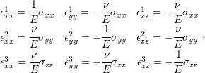 | (2.17) |
where the indexes xx, yy, and zz stand for the normal strains and stresses. The super-indexes 1, 2, and 3 refer to the deformations induced by forces in the x, y, and z directions, respectively.
Finally, all the strains in each direction can be superimposed (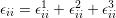 ) and
with some algebraic manipulation the final total strain in each direction is given
by
) and
with some algebraic manipulation the final total strain in each direction is given
by
 | (2.18) |
Regarding the shear components, the coefficient determination follows directly from the uniaxial Hooke’s Law. Similarly to the previous case, the shear stress relates to the strain by a coefficient as in
 | (2.19) |
where  and
and  are the shear stress and strain. G is the shear modulus and defines the
resistance of a body to torsion. The shear modulus can be written in terms of the Young
modulus and the Poisson ratio according to
are the shear stress and strain. G is the shear modulus and defines the
resistance of a body to torsion. The shear modulus can be written in terms of the Young
modulus and the Poisson ratio according to
 | (2.20) |
In conclusion, Hooke’s law with all constants is given by
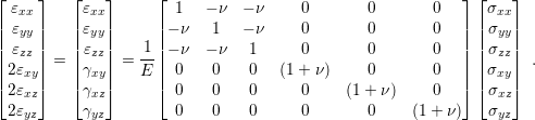 | (2.21) |
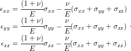
The inverse relation with the stress on the left side is written as
 | (2.22) |
 )
)