Next: 5.2 Impact of Gate Oxide Thickness Variations on HCD Up: 5. Analytic Modeling Approach for HCD Previous: 5. Analytic Modeling Approach for HCD
One of the manifestations of HCD is the linear drain current Idlin degradation. The Idlin change over time is a consequence of a large number of microscopic contributions. These contributions are related to the dangling bonds produced due to the Si-H bond dissociation. A dangling bond can capture a carrier, thereby producing a charged defect, which perturbs the electrostatics of a device and degrades the mobility. The driving force of the bond-breakage process is the energy deposited by carriers and thus the distribution of the energy describes the intensity of the bond dissociation mechanism. At the same time, the carrier ensemble evolves as it moves through the device. Physically this means that the carrier distribution function (and the acceleration integral) changes with the coordinate along the interface. Since the acceleration integral defines the characteristic time for trap creation, the interface states are distributed spatially and over the characteristic time. This time, in turn, describes the activation exponent and thus the dynamics of the defect generation process.
The analogous situation is typical for negative bias temperature instability where the dispersion of time constants (describing defect activation) stems from the distribution of the activation energy [136,192,193]. The mathematical formalism for this case was elaborated using the Fermi-Dirac function derivative as the probability density for the activation energy. This shape of the distribution leads to a power law dependence of the degrading parameter, see [40,194,195]. In the case of HCD the situation is more complicated because the activation of the Si-H bond dissociation process is triggered by the AI which is coordinate dependent, see Section 3.1. The bonds located at the coordinate corresponding to a smaller value of the AI will be broken later than those located near the drain end of the gate, i.e. near the typical AI peak. Therefore, one should consider the matter in terms of the distribution of the acceleration integral I(x) with the lateral coordinate x.
Based on the detailed model for HCD the acceleration integral is fitted with an analytical formula. Such an approach allows for the interface state density Nit and, hence, the degradation of the linear drain current, to be expressed analytically. One of the main features of this concept is that it is based on the physical principles behind HCD rather than on empirical fitting of experimental data. In particular, this means that the interplay between the single- and multiple-carrier mechanisms of the defect creation is considered by the model. This is very important because HCD tests are performed at accelerated conditions where carriers are rather hot. At real operation conditions, however, the voltages are lower, resulting in lower carrier energies. As a consequence, the role of the multiple-particle process is accelerated. Therefore, under real operating conditions the relative contribution of the latter mechanism is expected to be increased and the transition from stress to operating conditions may only be captured by a physics-based HCD model.
|
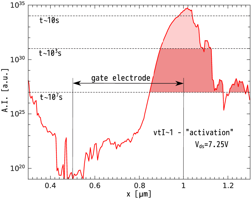
For these investigations a long-channel 5V n-MOSFET (sketched in Figure 3.2) designed on a standard 0.35um technology is employed. To ensure such a high operating voltage a thicker gate oxide (with an oxide thickness of 15nm), a longer channel thickness and special measures concerning the source/drain doping were undertaken. The devices have been subjected to hot-carrier stress for 104s at room temperature, using the gate voltage Vgs = 2.0V and 5 different drain voltages Vds = 6.25, 6.5, 6.75, 7.0, 7.25V. To calculate the carrier distribution function the proposed TCAD model I(x profile (calculated for Vds = 7.25V) is represented in Figure 5.1. This information will be further used as an additional verification data. Moreover, the information on I(x is crucial for the derivation of the analytical model because it will be based on fitting of this profile by an analytical expression. As an additional verification data input the dependence of the AI on the coordinate along the interface x, calculated with the TCAD model described in Section 3.1, is employed.
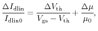
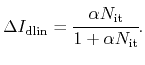
The linear drain current degradation due to Nit build-up is [30]where Idlin0 and μ0 are the linear drain current and mobility of the fresh device, respectively, and Δμ (ΔVth) is the change in mobility (threshold voltage). The mobility of the degraded device is calculated via (3.13). Relying on the experimental observation that, in the considered device ΔVth is weak, ΔIdlin and Nit are linked as
As in the TCAD version two competing mechanisms for Si-H bond-breakage are considered, i.e. the single-particle and multiple-particle processes [30]. The interface states generated by the SP-process are characterized by the density Nit,SP (see (3.3)) which is found by assuming first-order kinetics for the bond-breakage reaction. As shown in Section 3.1, the MP-related contribution is not coordinate-dependent because the acceleration integral reaches high values. Therefore, the density Nit,MP is not considered as a spatially distributed quantity.
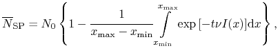
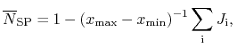
Since our aim is to develop an analytical model which does not use any information from the TCAD version (e.g. lateral profiles such as Nit(x) and I(x)), for the SP-process the average (over the interface) an effective trap concentration is introduced
with xmax and xmin as the boundaries of the Si/SiO2 interface. The integration over x captures all values of the AI. The probability that a Si-H bond is broken within a certain time period is given by (5.3). The coordinate-dependent acceleration integral I(x) defines the characteristic time of defect creation for each particular position along the interface.
(a)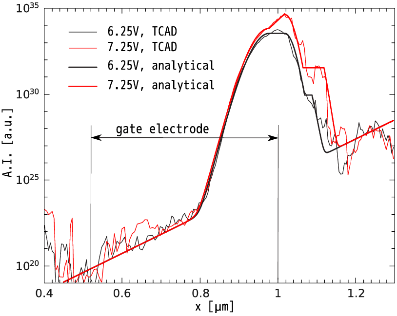 (b)
(b)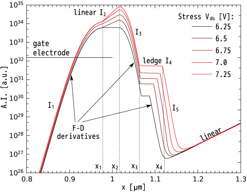
|
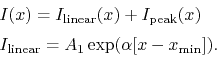
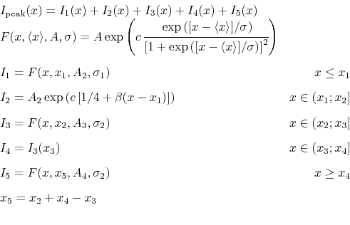
Figure 5.1 shows the AI profile I(x) for Vds = 7.25V which can be decomposed into two parts, i.e. the linear dependence (on a log-scale) on the coordinate Ilinear and the peak Ipeak, see Figure 5.1 and Figure 5.2a
The decaying line observed in the range 0.3...0.5um can be omitted because only bonds where the condition νtI~1 is satisfied have a significant probability to be broken; i.e. this fragment corresponds to the stress time 107s and the dissociation process is not triggered within the given time period. The slopes of the AI peak are well described by Fermi-Dirac derivatives on a log-scale. The peak of the AI is represented by piecewise functions, see Figure 5.1 and Figure 5.2b
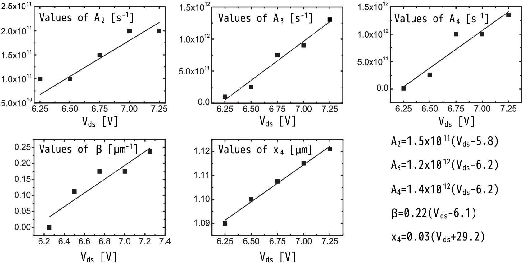 |
It can be observed (Figure 5.2a and Figure 5.2b) that the slope of the left front (i.e. I1) and the right front (I3 and I5 with the same σ2) do not vary with Vds. The position of the maxima of I1 and I3 (x1 and x2, respectively) remains the same with the increasing Vds and the only varying parameters are the slope of I2 (parameter β) and the extension of the ledge I4 (i.e. x4 - x3); the position of the I5 maximum is linked to the end of I4, see (5.5). The values of those parameters which vary with the stress Vds (i.e. fitting parameters of the model) are shown in Figure 5.3. Their variation with Vds can be represented by a linear dependence. Note that scattering in these parameters is related to the noise in the TCAD data, which is a consequence of the MC method employed for the solution of the Boltzmann transport equation. This circumstance allows for the calculate of the AI for those stress conditions for which the set of DFs has not been calculated. For this purpose values of must be interpolated/extrapolated {A2,A3,A4,β,x4} using the findings from Figure 5.3.
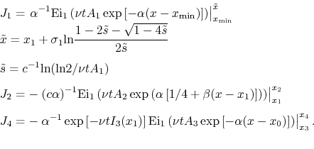
The full solution of (5.3) is written as where Ji is the contribution produced by the term Ii, i.e.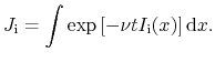 |
(5.7) |
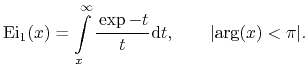
The terms Ji are expressed via the exponential integrals of the first kind Ei1(x) which is defined as [197]
The contributions Ji have the following structure (terms J3 and J5 are similar to J1 and thus are omitted here)
Figure 5.4a demonstrates the time dependences of the integrals Ji calculated for Vds = 7.25V. The terms Ji reflect the fraction of "virgin" bonds and a decay in Ji means that the dissociation process was triggered during this time period. It is evident that the "tip" of the AI peak (the term I2 of the AI and the J2 in ΔIdlin affects Idlin rather weakly already at t = 10s. In fact, I2 varies approximately in the range of 1034-1035a.u. (Figure 5.2a) and the criterion νtI1∼1 leads to bond-breakage events predominately triggered within the time period of 0.2s to 2s. In contrast, I1 varies by more than 11 orders of magnitude and thus J1 contributes to ΔIdlin over several decades and defines the degradation at long times. These considerations are summarized in Figure 5.4b where the time-dependent values of some Ji terms are substituted with constants. For instance, the term J1 does not substantially change during several decades (Figure 5.4a) and thus may be represented by the value J1(t=0). Figure 5.4b shows that during the time period of 0..104s terms {J2,J3,J5} are not significant and may be omitted.
(a)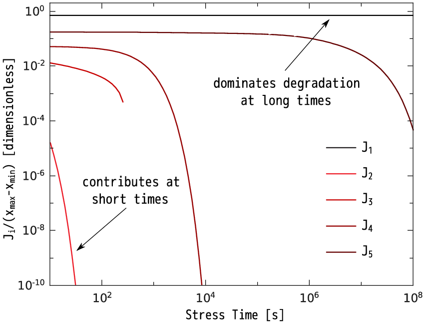 (b)
(b)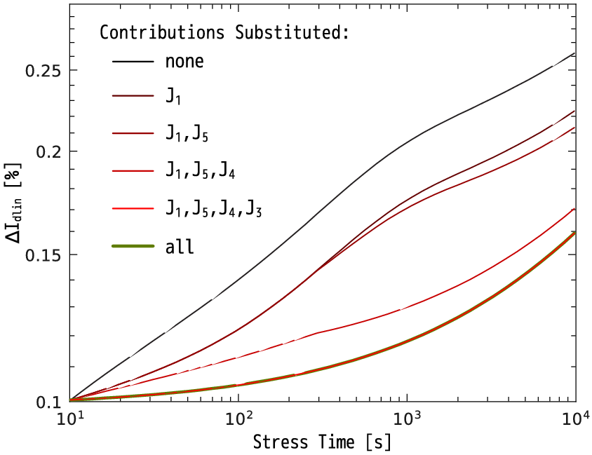
|
Since in the experiment it is impossible to separate the SP- and MP-components, one employs the TCAD model to show the Idlin degradation induced solely by the SP-mechanism. This step is important because it allows for the verification of the adequacy of the acceleration integral profile representation with a fitting formula. Figure 5.5a shows good agreement between the results calculated by TCAD and analytical models. The major discrepancy is observed at short times and is related to the noise seen in the AI peak and the related stochastic nature of the Monte-Carlo method.
Being sure that the SP-component is reasonably represented with the analytical expression the SP- and MP-contributions were combined. ΔIdlin considering also the MP-component is compared with experimental data and plotted in Figure 5.5b, which demonstrates a very good agreement between simulation and experiment.
(a)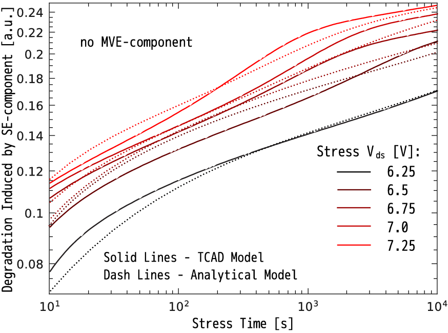 (b)
(b)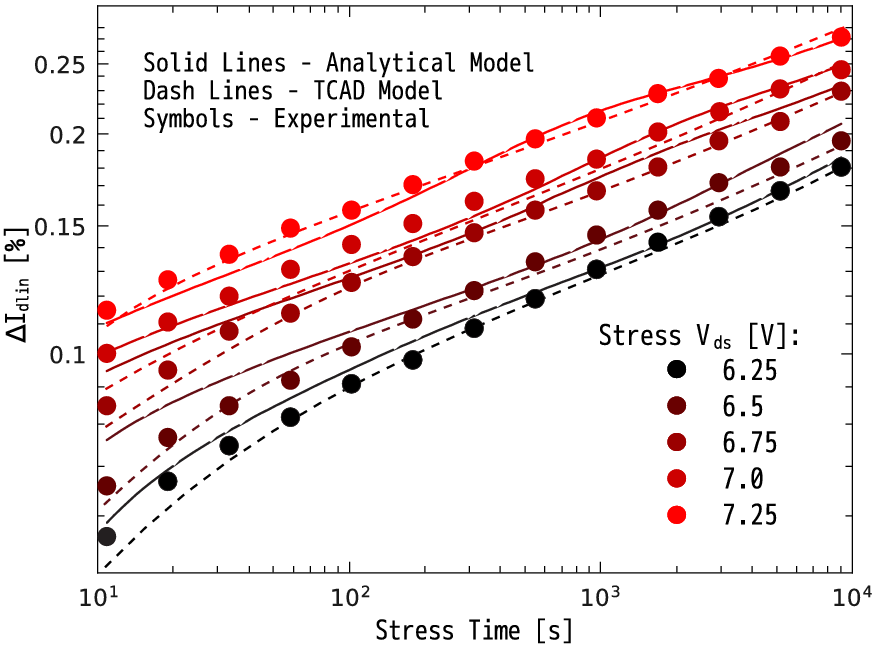
|
This model based on the analytical representation of the AI does not employ time consuming MC simulations required to calculate the set of carrier DFs. One may profit from such an advantage while considering the impact of statistical variations in device geometry (e.g. in the oxide thickness, gate length, etc) on HCD. If one should recalculate the entire set of carrier DFs with the MC method at each value of the fluctuating parameter, the simulation process will be inadmissibly time expensive. In contrast, within the developed model, the DFs are calculated only once for several reference values of the fluctuating quantity and the fitting parameters of the model (controlling the AI) are defined by interpolation using dependences such as those in Figure 5.3. Afterwards, one may use the analytical form of the AI and operate with simple expressions, which can be further weighted considering the distribution of the fluctuating quantity and statistically processed.