This section deals with the basic settings and configuration of the small-signal simulation mode. In addition, some information about the internal implementation is given. As transient and small-signal analysis are related simulation modes, their setup and configuration is very similar (see Appendix A.1).
The AC steps are based on a fully converged steady-state operating point, Therefore, it has to be ensured, that a DC simulation is started prior to any AC step. Note that this is also implicitly the case for transient simulations. During initialization of a transient or small-signal simulation, the internally used time or frequency representation is updated. Due to the backward Euler discretization the transient simulation mode requires the difference between two time points. Thus, in addition to the current time point also the last point has to be stored.
All models obtain the reciprocal time as input, which is used by the transient models to calculate their time-dependent contributions to the equation systems. Depending on the simulation mode, the variable contains either the reciprocal time difference or the angular frequency. Therefore, it is set as follows:
![\begin{gather*}\begin{split}r_{\mathrm{transient}} = \displaystyle\frac{1}{t_0 - t_1}\ , \\ [2mm] r_{\mathrm{ac}} = 2 \pi f\ . \end{split}\end{gather*}](img624.png) |
(3.13) |
This value is then passed to each model, indicating a DC step in case of zero and a transient or small-signal step in case of non-zero values. All models are subsequently called to add their contributions to the linear equation system. In order to excite the device, the user can specify the complex-valued amplitude of each terminal of the device.
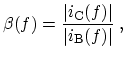
These standard small-signal capabilities will be demonstrated on a simple diode as shown in Figure 3.6. In the example discussed below, the capacitances over a wide range of frequencies are extracted. The anode voltage is an additional parameter of the simulation. Refer to Appendix A.3 for further details on the simulation setup.
![\includegraphics[height=0.28\linewidth]{figures/simple_diode2.eps}](img625.png)
![\includegraphics[height=0.28\linewidth]{figures/cut2.eps}](img626.png)
|
In addition, the diode was also subject to transient simulations in order to
demonstrate the generation of harmonics when the device is excited with large
signals. Three different amplitudes ![]() were used in the signal applied at the
amplitude:
were used in the signal applied at the
amplitude:
| (3.14) |
The upper left side of Figure 3.8 shows the comparison of the
simulation results with those obtained by the commercial simulator DESSIS
[111]. The other three figures compare small-signal and transient
simulation results of MINIMOS-NT. For an anode voltage of ![]() V, both modes
are used to extract the capacitances and arguments. In the lower right figure
the simulation effort and the relative error of the transient results in
comparison to those obtained by the small-signal mode are shown. It is
important to note that the transient mode requires more than twice the time of
the small-signal mode for only ten steps. For 1000 transient steps, the effort
is more than 60 times larger than for the small-signal simulation.
V, both modes
are used to extract the capacitances and arguments. In the lower right figure
the simulation effort and the relative error of the transient results in
comparison to those obtained by the small-signal mode are shown. It is
important to note that the transient mode requires more than twice the time of
the small-signal mode for only ten steps. For 1000 transient steps, the effort
is more than 60 times larger than for the small-signal simulation.
![\includegraphics[width=0.49\linewidth ]{figures/fft1_3.eps}](img637.png)
![\includegraphics[width=0.49\linewidth ]{figures/fft500_3.eps}](img638.png)
![\includegraphics[width=0.49\linewidth ]{figures/fft250_3.eps}](img639.png)
![\includegraphics[width=0.49\linewidth ]{figures/fft10_3.eps}](img640.png)
|
![\includegraphics[width=0.49\linewidth ]{figures/diode_dessis.eps}](img641.png)
![\includegraphics[width=0.49\linewidth ]{figures/diode_cabs2.eps}](img642.png)
![\includegraphics[width=0.49\linewidth ]{figures/diode_carg3.eps}](img643.png)
![\includegraphics[width=0.49\linewidth ]{figures/diode_erel3.eps}](img644.png) |
Frequency stepping can be based on several approaches (see
Section 3.1.3). One possibility is to apply a conditional stepping
algorithm which is directly stepping to the unity gain point. Such a method is
not only faster and more accurate, but additionally makes a post-processing for
interpolations or extrapolations obsolete. As for a bipolar transistor ![]() is defined as
is defined as
 |
(3.15) |
The objective of the conditional stepping is to find the root of the function (3.16) with an error below a specified value. As such a simulator capability can be applied to extract also other quantities, for example the threshold voltage, it is generally implemented and derived in the following.
Basically, the root of the nonlinear function ![]() is bracketed in the interval
is bracketed in the interval
![]() . The values
. The values
![]() and
and
![]() have opposite signs and the
function is continuous, for that reason one root lies in the interval
given. The conditional stepping algorithm is based on the well-known
Regula Falsi (False Position) algorithm. According to
[165] the nonlinear function is assumed to be approximately linear in
the local region of interest.
have opposite signs and the
function is continuous, for that reason one root lies in the interval
given. The conditional stepping algorithm is based on the well-known
Regula Falsi (False Position) algorithm. According to
[165] the nonlinear function is assumed to be approximately linear in
the local region of interest.
False Position converges less rapidly than the related Secant method. In contrast to a Newton method which requires the derivatives, only the actual function values are used. For that reason, the algorithm can be directly integrated in the respective stepping module (see Appendix B).
The first two iteration steps are used to obtain the initial values
![]() and
and
![]() at the specified start boundaries
at the specified start boundaries
![]() (lower boundary) and
(lower boundary) and
![]() . These values must have opposite signs, otherwise the method fails. The
next value is found at the intersection of the line connecting these two
points. This line is given by
. These values must have opposite signs, otherwise the method fails. The
next value is found at the intersection of the line connecting these two
points. This line is given by ![]() :
:
 |
(3.17) |
Depending on the sign of
![]() either the lower or the upper boundary is
replaced by
either the lower or the upper boundary is
replaced by
![]() . The loop is terminated if
. The loop is terminated if
![]() is smaller than the
accuracy given or if the maximum iteration count is reached.
is smaller than the
accuracy given or if the maximum iteration count is reached.
For
![]() extraction this algorithm seems to be promising as the frequency
characteristics are indeed an approximately linear function (in the area of
interest) with only one root. However, an important drawback of this approach
is the use of fixed boundaries
extraction this algorithm seems to be promising as the frequency
characteristics are indeed an approximately linear function (in the area of
interest) with only one root. However, an important drawback of this approach
is the use of fixed boundaries
![]() and
and
![]() . First, the frequency range of a
. First, the frequency range of a
![]() extraction can be very wide, especially if more than one operating point
is required. Second, the method fails if both values
extraction can be very wide, especially if more than one operating point
is required. Second, the method fails if both values
![]() and
and
![]() have the
same sign. Third, the method converges slowly if the interval
have the
same sign. Third, the method converges slowly if the interval
![]() is very wide. To overcome this trade-off between usability and performance, the
boundaries
is very wide. To overcome this trade-off between usability and performance, the
boundaries
![]() and
and
![]() are always reread during the simulation. Furthermore, an
automatic adaptation is provided such that too narrow boundaries are
automatically extended. This allows on the one hand side the specification of
very narrow boundaries, which is important to speed up the convergence, and
exempt the user of finding practicable values for
are always reread during the simulation. Furthermore, an
automatic adaptation is provided such that too narrow boundaries are
automatically extended. This allows on the one hand side the specification of
very narrow boundaries, which is important to speed up the convergence, and
exempt the user of finding practicable values for
![]() and
and
![]() , which can be a
cumbersome task.
, which can be a
cumbersome task.
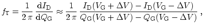
In order to quantify these considerations, an evaluation of various boundary
settings and error values has been performed. The narrowness of the boundaries
![]() in respect of an
in respect of an
![]() (which is already known) means, that the lower and
upper boundaries equal
(which is already known) means, that the lower and
upper boundaries equal
![]() , respectively (
, respectively (
![]() GHz). In
Figure 3.9 the effort for the extraction of
GHz). In
Figure 3.9 the effort for the extraction of
![]() in terms of the
required steps is analyzed. The left figure shows the iteration steps for two
different sets of boundaries. The right figure compares various boundaries and
errors. It can be seen that a significant speed-up can be achieved with narrow
boundaries even for very accurate simulations.
in terms of the
required steps is analyzed. The left figure shows the iteration steps for two
different sets of boundaries. The right figure compares various boundaries and
errors. It can be seen that a significant speed-up can be achieved with narrow
boundaries even for very accurate simulations.
![\includegraphics[width=0.49\linewidth ]{figures/ft_cond.eps}](img660.png)
![\includegraphics[width=0.49\linewidth ]{figures/ft_steps.eps}](img661.png)
|
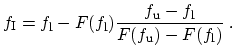
In Figure 3.10, extracted cut-off frequencies for MOS transistors with different gate lengths and the three transport models as discussed in Chapter 2 are shown. The results obtained by the small-signal simulation mode of MINIMOS-NT are compared with Monte Carlo data [83] and results based on the quasi-static approximation. The latter are obtained as a result of steady-state simulations. By applying the quasi-static approximation, the following definition can be used for MOS transistors [115,217]:
![\includegraphics[width=0.49\linewidth ]{figures/ft2.eps}](img664.png)
![\includegraphics[width=0.49\linewidth ]{figures/ftfull2.eps}](img665.png)
|
![\includegraphics[width=\linewidth]{figures/time.eps}](img636.png)