By comparing saved MCSR structures of the same system matrix assembled by the formerly used and the new module, misordering problems have been detected. As a consequence, the new modules were presumed to deliver wrong results and an investigation of the problem was started which finally resulted in an elegant solution for the problem which is directly related to the row transformation.
The row transformation as discussed in Section 4.7.1 is used to supply equations (or rows of the system matrix) with equations having a higher priority. This is necessary, because several segments (with different priorities) could contain the same grid point. Each of the control functions determines a result for this grid point, but only the one with the highest priority should be used.
See Figure 4.6 for an illustration of the physical background as it occurs for a MOS structure. The semiconductor segment (segment 1), the gate oxide (segment 2), and the source contact (segment 3) share one physical grid point. Thus, three equations are assembled to obtain the solution for the potential at this point.
Since the contact segment has the highest priority, its solution has to
be used by the other two segments. However, during the assembly of the
three interface equations, the interface models (which are responsible
for setting up the transformation matrix), do not have the full
information about all three segments involved. They only take two
segments into account, namely the segments the interface is
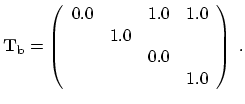
in-between. As a consequence, the following transformation entries can
be found in
![]() :
:
These transformations result in the following equations of the complete linear
equation system. Depending whether a correction is activated or not, equation 3
is shown in (4.27) and (4.28), respectively. ![]() stand for
other contributions equal for both cases and thus not of interest here. The
coefficients
stand for
other contributions equal for both cases and thus not of interest here. The
coefficients ![]() denote entries wrongly transferred to (4.30)
instead of (4.27). With
denote entries wrongly transferred to (4.30)
instead of (4.27). With
![]() as the contact potential
of segment 3 (source contact), the correct and wrong equation 115 can be seen
in (4.29) and (4.30), respectively:
as the contact potential
of segment 3 (source contact), the correct and wrong equation 115 can be seen
in (4.29) and (4.30), respectively:
Since the segment equation should also be transferred to the equation of the boundary charge, the red/ dashed transformation is wrong and should be replaced by the green/thick one. As a consequence, the gate oxide is transferring its incomplete equation to the semiconductor segment. Such situations could be prevented if the respective models are provided with the complete information. Since this is not the case for the main simulator MINIMOS-NT and for unstructured meshes an arbitrary number of segments would have to be considered, the assembly module was equipped with an algorithm which corrects the transformation matrix before it is applied. This algorithm has the full information available, but remains deactivated for all simulators which do not require this correction. See Table 4.3 for a comparison of the terminal quantities showing significant differences particularly for the boundary charge.
The reason for the differences between the formerly used and new module can be explained as follows: one important difference between the modules is the assembly sequence. The new assembly module assembles four matrices and compiles them afterwards to the complete linear system (see Section 4.14). This compiling step uses matrix additions and multiplications which operate on the completely assembled structures.
In contrast, the formerly used module calculates all transformations during a symbolic assembly phase in advance and is therefore able to assembly only one system matrix during the actual assembly phase (cf. Newton adjustment). So the matrix additions and multiplications are performed immediately while an entry is added. As analyzed, these transformations do not perform a multiplication in the strict mathematical form, but are already adapted for the requirements described above. This behavior should be demonstrated on a simple mathematical example.
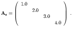
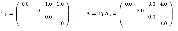
For the demonstration of the matrix transformation, consider a simple
![]() matrix multiplied by
matrix multiplied by
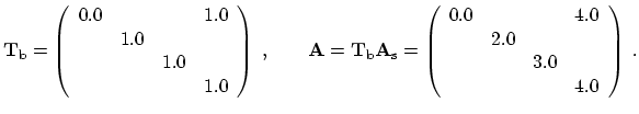
![]() from the left:
from the left:
| (4.31) | |
 |
(4.32) |
 |
(4.33) |
The second transformation matrix and the multiplication result are:
The third transformation matrix and the multiplication result are:
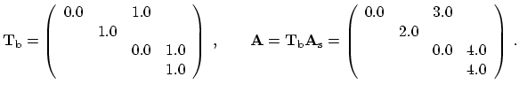 |
(4.35) |
As discussed above, the formerly used module takes such situations into account while calculating all contributions of a matrix entry. However, the new assembly module requires a correction algorithm before the mathematically correct matrix multiplication is processed during the compiling process. For the following reasons, the development of a correction algorithm is a crucial part for the success of the new modules:
For these reasons, it was decided to develop a correction algorithm which is presented here. Based on the third example in the last section, the problem is described verbally once again: equation three is transformed to equation two, that is transformed itself to equation zero: thus, a transformation source is also a transformation target. A correction to replace the (three to two to zero) problem by a straightforward (three to zero) transformation is required.
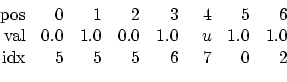
The basic correction algorithm can use all information provided by the
transposed MCSR data structure. In
![]() , the column indices
represent the targets of the transformations.
, the column indices
represent the targets of the transformations.
 |
(4.36) |
 |
| (4.37) |
![$\displaystyle \mathrm{idx}[\underbrace{\mathrm{idx}[5]}_{0}] = \mathrm{idx}[\underbrace{\mathrm{idx}[5] + 1}_{1}] = 1 \ .$](img838.png) |
(4.38) |
![$\displaystyle \overbrace{\mathrm{idx}[\underbrace{\mathrm{idx}[6]}_{2}]}^{5} \neq \overbrace{\mathrm{idx}[\underbrace{\mathrm{idx}[6] + 1}_{3}]}^{6} \ .$](img839.png) |
(4.39) |
| (4.40) |
| (4.41) | |
![$\displaystyle \mathrm{idx}[6] = \mathrm{idx}[\underbrace{\mathrm{idx}[\overbrace{\mathrm{idx}[6]}^{2}]}_{5}] = 0\ .$](img842.png) |
(4.42) |
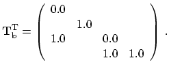
After the correction is completed,
![]() has to be transposed back
resulting in the same transformation matrix as used in (4.34):
has to be transposed back
resulting in the same transformation matrix as used in (4.34):
 |
(4.43) |
The basic algorithm explained above could not be used for more complicated structures, for example the ones which contain grid points calculated by four control functions.
In addition, duplicate entries in the resulting MCSR structure (as they could occur using the basic algorithm) should be avoided. In contrast to the full format, a sparse format stores only entries which are intended to be non-zero. Besides the actual value, also the row and column number have to be stored. Thus, it is possible to store one matrix entry more than one time, which is a duplicate entry of the same position. Most of the mathematical operations defined for MCSR take those implicitly into account, since they simply process all entries in the structure. However, due to the fact that all multiple entries should be actually summed up to one entry, numerical inaccuracies may occur. So duplicate entries are best avoided at all.
The main objective of the advanced algorithm should provide a
generally applicable correction of the transformation matrix while
avoiding duplicate entries.
A new example should demonstrate the actual problem. In a transposed
transformation matrix
![]() the entries (row:34, col:3) and (47, 34)
are set to one. The basic algorithm corrects the latter entry to
(47, 3). Since there is only one entry, this correction is successful
(case one).
the entries (row:34, col:3) and (47, 34)
are set to one. The basic algorithm corrects the latter entry to
(47, 3). Since there is only one entry, this correction is successful
(case one).
To extend the example, an additional entry in (78, 34) is supposed to
be one. That means, that equation 34 is not only transferred to
equation 3, but also to equation 78. Note that in
![]() the column
index stands for the target of a transformation. In that case, the
basic algorithm fails, because there is not enough space to add new
entries (case two). Both cases are graphically represented in
Figure 4.7.
the column
index stands for the target of a transformation. In that case, the
basic algorithm fails, because there is not enough space to add new
entries (case two). Both cases are graphically represented in
Figure 4.7.
The first case is shown in Figure 4.7a and Figure 4.7b. In Figure 4.7a, two arrows represent two transformations, the blue/dashed arrow has to be redirected to the position the black/solid arrow points to. In Figure 4.7b, the green/dashed arrow represents the redirection. After the correction the number of arrows stays the same.
The second case is shown in Figure 4.7c and Figure 4.7d. Since
the center position is transferred to multiple (here two, generally ![]() ) right
positions, there are also
) right
positions, there are also ![]() arrows needed to point from the left position to
all right positions. The number of arrows increases by
arrows needed to point from the left position to
all right positions. The number of arrows increases by ![]() . In
Figure 4.7d, the red/dotted arrow has to be created additionally. In the
existing MCSR structure, there is no space for this entry. Hence, no
thorough correction of the second case could be made.
. In
Figure 4.7d, the red/dotted arrow has to be created additionally. In the
existing MCSR structure, there is no space for this entry. Hence, no
thorough correction of the second case could be made.
If equation 47 of
![]() contains the non-zero column entries 49, 51, and 55,
the following misorderings are the result of the omitted correction:
contains the non-zero column entries 49, 51, and 55,
the following misorderings are the result of the omitted correction:
For that reason new entries have to be added in order to completely correct the transformation matrix. There are two solutions for this problem:
By pursuing the second approach, an algorithm was developed which benefits from already existing and applied implementations. The system can now take all possible situations into account since it does not limit the number of commonly used grid points (independent of the number of spatial dimensions) any more. Table 4.4 summarizes the initial situation and the correction result for both the transposed and untransposed transformation matrix.
Regarding the Newton adjustment it is important to note, that the
advanced algorithm is fully employable due to the following
considerations. After a successful first Newton adjustment level,
no flexible sparse structure exists which could be used to add
additional entries. However, the already existing
![]() matrix does
already contain all required entries. This assumption holds since all
deterministic algorithms always yield the same result for the same
inputs. Therefore, no Newton adjustment errors will occur.
matrix does
already contain all required entries. This assumption holds since all
deterministic algorithms always yield the same result for the same
inputs. Therefore, no Newton adjustment errors will occur.
![\includegraphics[width=10.8cm]{figures/transfer2.eps}](img801.png)
![\includegraphics[width=10.8cm]{figures/trfgraph.eps}](img844.png)