![[*]](cross_ref_motif.gif) .)
A more accurate model for the capacitance of an island is the capacitance of
two or more spheres in a
line. A calculation for characteristic spatial dimensions shows an
increase of about 15% of the total capacitance. See
Appendix A for a detailed outline of
the calculations,
numerical results, and the description of an algorithm to calculate the
capacitance of an arbitrary arrangement of spheres. A collection of practical
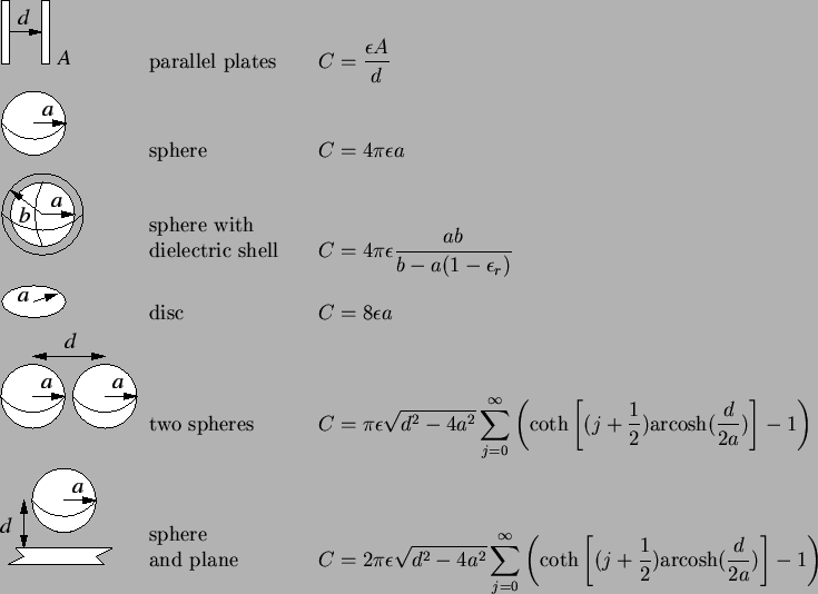
analytical capacitance formulas is given in Table 2.1.
.)
A more accurate model for the capacitance of an island is the capacitance of
two or more spheres in a
line. A calculation for characteristic spatial dimensions shows an
increase of about 15% of the total capacitance. See
Appendix A for a detailed outline of
the calculations,
numerical results, and the description of an algorithm to calculate the
capacitance of an arbitrary arrangement of spheres. A collection of practical
analytical capacitance formulas is given in Table 2.1.
 |
Systems with sufficiently small islands are not adequately described with this
model. They exhibit a second electron-electron interaction energy,
namely the change in
Fermi energy, when charged
with a single electron. One
must distinguish between metals and semiconductors, because of their greatly
different free carrier concentrations and the
presence of a band gap in the case
of semiconductors. Metals have typically a
carrier concentration of
several
![]() and undoped Si about
and undoped Si about
![]() at room temperature (see Material Properties
Table ).
The low intrinsic carrier concentration for semiconductors is in reality not
achievable, because of the ubiquitous impurities which are ionized at room
temperature. These impurities supply free charge carriers and may lift the
concentration, in the case of Si,
to around
at room temperature (see Material Properties
Table ).
The low intrinsic carrier concentration for semiconductors is in reality not
achievable, because of the ubiquitous impurities which are ionized at room
temperature. These impurities supply free charge carriers and may lift the
concentration, in the case of Si,
to around
![]() ,
still many orders of
magnitude smaller than for metals. Clearly, doping increases the carrier
concentration considerably, and can lead in the case of degenerated
semiconductors
to metal like behavior. We are considering only undoped semiconductors to
emphasize the difference to metals.
,
still many orders of
magnitude smaller than for metals. Clearly, doping increases the carrier
concentration considerably, and can lead in the case of degenerated
semiconductors
to metal like behavior. We are considering only undoped semiconductors to
emphasize the difference to metals.
The dependence of the Fermi energy EF on carrier concentration n is
derived
in Appendix B
(see also [7]). For metals it is given by
![]()
and for semiconductors it is
![]()
where
![]() is the net carrier concentration defined as
is the net carrier concentration defined as
![]() .
Fig. 2.1 compares the change in the Fermi energy for the addition
of one, two, and three electrons in Si to the electrostatic charging energy.
.
Fig. 2.1 compares the change in the Fermi energy for the addition
of one, two, and three electrons in Si to the electrostatic charging energy.
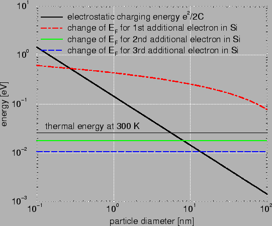 |
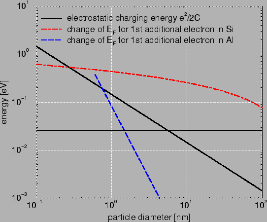
Fig. 2.2 compares Si with Al. It is clearly visible that the change
is much bigger in Si. This is caused by two reasons. First, the difference in
free carrier concentration. In metals much more carriers are available and
therefore
the addition of one electron has not such a big impact anymore. Second in
metals an additional electron finds a place slightly
above the Fermi level. In semiconductors due to the energy gap the electron
needs to be inserted considerably above the Fermi level.
 |