Subsections

• 3.4.1 Least Squares Fitting of the Model Function
• 3.4.2 Propaedeutic Example

3.4 Hessian Refinement Method

The idea behind the Hessian refinement method is to use the Hessian matrix, calculated for a given scalar data field $f(x,y,z)$ , stored on the initial mesh, for the anisotropic metric function $\mathbf{M}$ , which is used for the anisotropic tetrahedral bisection algorithm.

The Hessian $\mathbf{H}$ for a three-dimensional function $f(x,y,z)$ with non-zero second derivatives is given by

$$\mathbf{H}:=\begin{pmatrix}\frac{{\rule[0.0mm]{0mm}{\Myhi}\displa... ...(x,y,z)}}{{\rule[0.0mm]{0mm}{\Myhi}\displaystyle\partial z^{2}}} \end{pmatrix}.$$ (3.18)

In general the entries of the Hessian matrix are possibly negative or may be zero. For the usage of the Hessian as metric for the refinement strategy, a transformation has to be performed. This transformation is done simply with the norm of all function derivatives and offsetting by the identity matrix. The corresponding matrix can be written as

$$\mathbf{m}_{ij} = \delta_{ij} + \vert\mathbf{h}_{ij}\vert\quad (i,j = 1,2,3) \quad \delta_{ij} = \begin{cases}0& \quad \text{if} \quad i \neq j \ 1& \quad \text{if} \quad i = j \end{cases}$$ (3.19)

To scale the metric function a scalar factor $k$ is used. This factor describes the maximum edge length in a static non-biased metric space, with $\mathbf{M} \equiv \mathbf{I}$ the identity matrix. The advantage of using the Hessian matrix is that it excellently reflects the curvature of the iso-levels of an initial scalar data function $f(x,y,z)$ and guarantees a good approximation in regions with high second derivatives [49].

Since the scalar function $f(x,y,z)$ is not known analytically, which is almost the case for numerical calculations in TCAD tools, a method has to be found, where a local approximation of the Hessian matrix can be defined. Linear interpolation via the linear weighting functions (as depicted in Equation 3.7) is not practicable, as the piecewise constant gradient cannot be derived any more. Based on the scalar data function values stored on the 0 -faces of the mesh which gives a scattered data distribution (scalar data 0 -face relation, cf. Figure 3.2(a)) a method is derived which allows to calculate an estimation of the Hessian matrix based on a least squares fit of an three-dimensional model function.

3.4.1 Least Squares Fitting of the Model Function

For the fitting of a model function to some given scattered data, a function is used which measures the closeness between the data and the model function and determines all parameters of the model function for a best fit. An established method for this task is so-called least squares fitting which is is a procedure for finding the best-fitting curve by minimizing the sum of the squares of the offsets, the so-called residuals, of the data points from the curve [61].

The choice of a proper model function is difficult, because in general the characteristic of the scattered data function is not known. Based on the definition of the Hessian matrix, the model function should be continuous, twice differentiable and sufficiently smooth. Preliminary experiments have shown that model functions with the characteristics of a Gaussian bell curve fulfill these requirements.

On this note, the following model function is used as local approximation function of the scattered scalar data, stored on the mesh:

$$u_M(x,y,z)=e^{k} e^{-a(x-x_{0})^{2}} e^{-b(y-y_{0})^{2}}e^{-c(z-z_{0})^{2}},$$ (3.20)

where the fitting parameter set $\{k,a,b,c,x_0,y_0,z_0\}$ has to be determined by the means of the linear least squares method. In Appendix B.2 a brief introduction of the linear least squares method is given, which is a summary of articles in [62,63].

The determination of the fitting parameter set $\{k,a,b,c,x_0,y_0,z_0\}$ is performed pointwise, i.e. for every vertex in the mesh a different set is calculated. For the parameter set the degrees of freedom is seven, which is the minimum of scattered data points to be considered. For the calculation of the fitting parameters related to a particular vertex the nearby vertices of this vertex have to be taken into account. This can be carried out by looking at all vertices which are connected to the particular vertex via edges, this is the so-called point batch of the particular vertex. If this does not yield enough data points, the point batch has to be extended by the point batches of all the points of the initial point batch and so on, for instance.

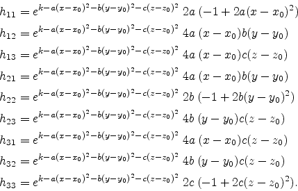
The Hessian matrix can now be calculated from the model function $u_M$ given by Equation (3.20), which is a continuous approximation of the scattered scalar data function and afterwards used as anisotropy metric tensor function for the anisotropic tetrahedral bisection algorithm. Since the set $\{k,a,b,c,x_0,y_0,z_0\}$ is determined locally for each vertex, the Hessian is also defined for each vertex. With respect to the model function $u_M(x,y,z)$ the Hessian is given by

$$\begin{split}h_{11} &= e^{k-a(x-x_0)^2- b(y-y_0)^2-c(z-z_0)^2... ...2- b(y-y_0)^2-c(z-z_0)^2} 2c (-1+ 2c(z-z_0)^2). \end{split}$$ (3.21)

For the metric tensor function and the anisotropic line length calculation, see Equation (2.2), the pointwise defined metric via the Hessian matrix is kept constant up to the middle of the edge. This is shown in Figure 3.12 for two mesh points $P_1$ and $P_2$ with the constant metric functions $M_1$ and $M_2$ and their region of validity.

Figure 3.12: For the Hessian refinement strategy the metric tensor function $M(x,y,z)$ is defined pointwise. For the anisotropic edge length calculation the edge is split into two parts each with constant metric.

3.4.2 Propaedeutic Example

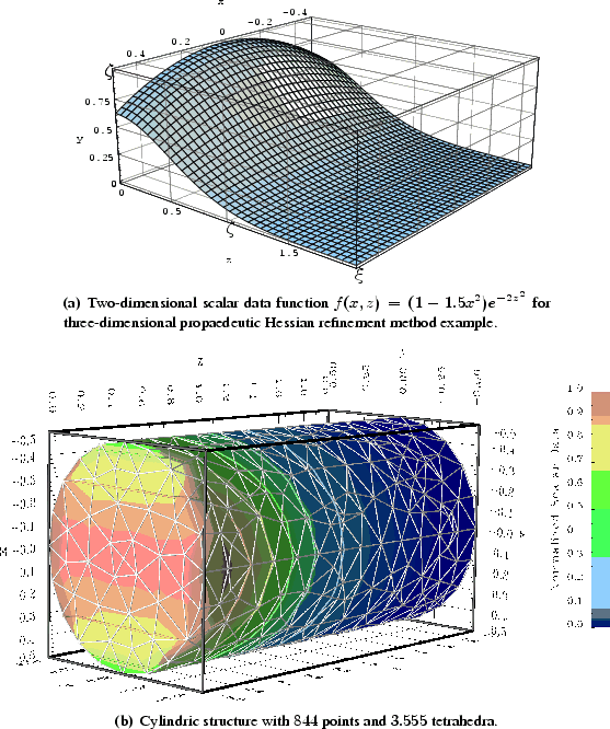
To see the Hessian refinement method in action, an example was chosen, where an initial three-dimensional cylindric tetrahedral mesh structure holds a two-dimensional scalar data distribution $f(x,z)$ given analytically for this propaedeutic example. The scalar data distribution reads to

$$f(x,z) = (1 - 1.5x^2)e^{-2z^2}.$$ (3.22)

A plot of this function $f(x,z)$ over the used range for $x$ and $z$ is depicted in Figure 3.13(a).

Figure 3.13: Figure 3.13(a) shows a plot of the two-dimensional scalar data distribution which is applied to the three-dimensional cylindric tetrahedral mesh structure, depicted in Figure 3.13(b).

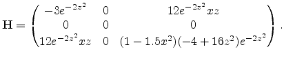
In this exceptional case we are in the lucky position that the scalar data function is given analytically which allows a direct calculation of the Hessian matrix. For the later-on presented results, of course, the approximation via the model function $u_M(x,y,z)$ , see Equation (3.20), as described in Section 3.4.1 was used.

However, the Hessian for the function given in Equation (3.22) reads to:

$$\mathbf{H}=\begin{pmatrix}-3e^{-2z^2} & 0 & 12e^{-2z^2}xz \ 0 & 0 & 0 \ 12e^{-2z^2}xz & 0 & (1-1.5x^2)(-4+16z^2)e^{-2z^2} \end{pmatrix}.$$ (3.23)

The evaluation, with respect to Equation (3.19), of the transformed Hessian for three particular points $p_1=(0,0,0)^T$ , $p_2=(0,0,1)^T$ , and $p_3=(0,0,2)^T$ is depicted in Figure 3.14. Please notice that the spatial expansion of the ellipsoidal glyph are scaled. The blue ellipsoid at $p_3$ is almost a sphere, since the entries of the Hessian given in Equation (3.23) are almost zero for this point, and as described in the beginning of Section 3.4, for the metric definition, the Hessian is offset by the identity matrix.

Figure 3.14: Metric function evaluation of the propaedeutic example structure. The ellipsoidal glyphs are scaled for a proper visualization. The blue ellipsoid at $p=(0,0,2)^T$ is almost a sphere, since the entries of the Hessian given in Equation (3.23) are nearly zero for this point, but for the metric definition, the Hessian is offset by the identity matrix. Therefore the semiaxis of the ellipsoidal glyph are approximately unity.

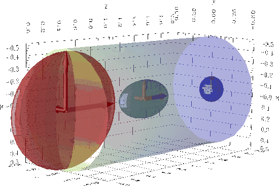In Figure 3.14 one can clearly observe, that the refinement is directionally oriented so that there is no dilation along the $y$ -axis. Along the positive $z$ -direction the intensity decreases to almost zero at $z=2$ . This behavior can also be observed along the $x$ -axis. For the refinement only regions are relevant where the ellipsoidal glyph representation of the metric function have semiaxis larger than unity . Based on this note one can expect significant refinement only for the region $z=0$ to $z=1.2$ . The refinement does not influence edge lengths along the $y$ -axis. For a first guess the intensity of the refinement at the point $p=(0,0,0)^T$ along the $x$ -axis is of the same strength as that given for the $z$ -axis. Therefore one can expect approximately the same mesh density along the $x$ - and $z$ -axis in this region.

For the following results the Hessian matrix is calculated by a least squares fit of a model function which shows the form of a three-dimensional Gaussian bell curve, described in Section 3.4.1. It is in the nature of this approach that the approximated Hessian shows slight differences compared to the proper definition given in Equation 3.18, since the scalar data function is usually not known analytically.

Figure 3.15: The Hessian refinement method was used to obtain an anisotropic refinement in regions of high second derivatives of the initial data profile. The mesh is untouched in regions with smooth iso-levels and the anisotropic orientation is aligned according to the curvature of the iso-level surfaces.

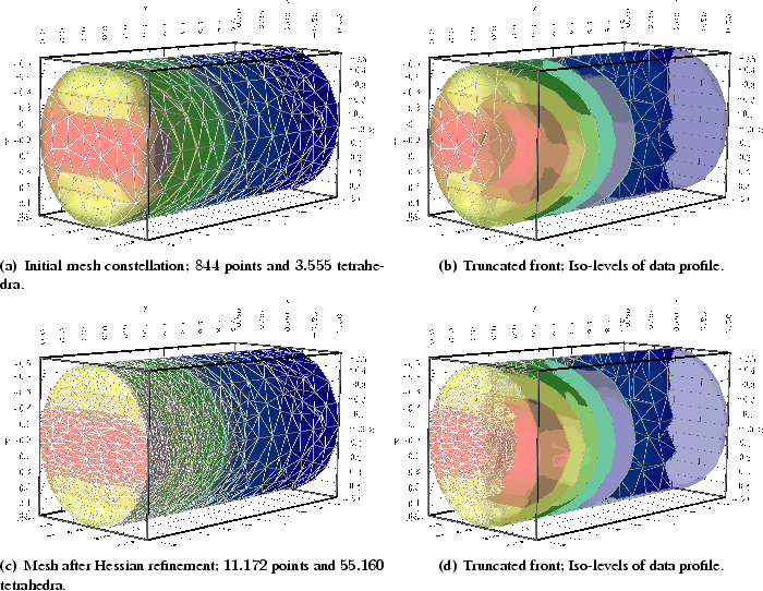Figure 3.15 gives an overview of the initial and refined mesh constellation. The upper left picture depicts the initial coarse cylindric mesh structure, and the corresponding right picture shows additional iso-levels of the scalar data distribution. The curvature of the iso-surfaces decreases with increasing spatial $z$ coordinates and shows almost no curvature along the $y$ -axis. To see both, the mesh and the iso-surfaces, the mesh structure is fractionalized in the way that for negative $y$ values only a couple of iso-surfaces are visible.

The second row shows the same pictures for the Hessian refined structure. Again, Figure 3.15(c) depicts the whole mesh structure and the according right picture gives the truncated part with the iso-surfaces. One can clearly observe that the $y$ direction is influenced only slightly by the refinement and shows almost a coarse mesh density, different to the mesh density along the $z$ - and the $x$ -direction, which gives a most regular structure in regions of low $z$ values. With increasing $z$ values the mesh density decreases up to regions beyond $z=1.2$ which are not influenced by the refinement.

Figure 3.16: One quarter of the refined structure in an orthographic view. The iso-surfaces are drawn end-to-end. One can clearly see that the refinement is restricted to regions where the iso-surfaces have a high curvature.

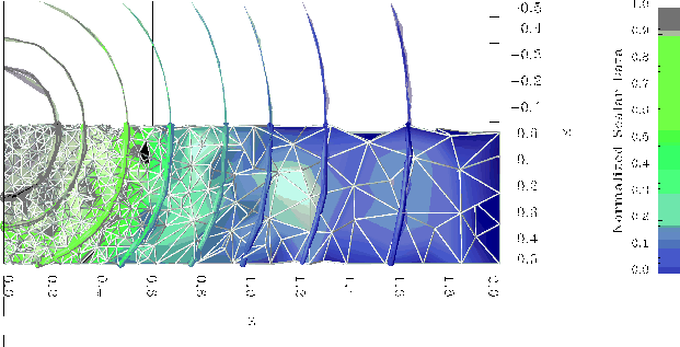Figure 3.16 gives an orthographic view of one quarter of the refined mesh structure. Here again the mesh is fractionalized to see the shape of the mesh elements. In this picture one can clearly see, that the refinement follows the curvature of the iso-surfaces and leaves regions with flat surface levels untouched.