4.3 A Further Diffusion Example

In Section 4.2 an exceptional example was presented where a one-dimensional diffusion problem was calculated on a three-dimensional test structure. In the following also a diffusion example is presented for which the solution is not available analytically. Again a Hessian refinement method, as described in Section 3.4 in combination with the error estimator presented in Section 4.1, is used to improve the overall accuracy of the simulation.

Figure 4.6: Initial diffusion simulation domain, a silicon block is partially covered by a silicon nitride mask. For the diffusion simulation a non-vanishing normal derivative of the dopant concentration was applied to the upturn part of the silicon block, marked with red arrows.

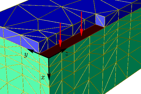Figure 4.6 shows the simulation setup where a cuboid block (green colored) is almost completely covered by a mask (blue colored) on top. Only a small band which is colored dark red is exposed to an ambient gaseous dopant source. The underlying initial mesh is a coarse, fairly isotropic mesh. At the upturn open part of the structure (colored dark red), a boundary condition with a non-vanishing derivative of the dopant concentration was applied, marked with $x$ -directional red arrows. This setup illustrates a $x$ -directional flux where dopants continuously arrives at the surface such that the concentration gradient remains constant at the surface [82].

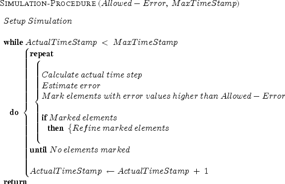
For the simulation procedure itself a combination of Hessian refinement and error estimation was applied. After every time step of the simulation the accuracy is checked with the error estimator and a refinement cycle is introduced on demand. Table 4.1 gives a pseudo code fragment which illustrates such a simulation procedure. The presented simulation cycle guarantees also that only regions of high error are refined, because only tetrahedra which are marked by the error estimator are influenced by the Hessian refinement, other regions are completely untouched.

The Hessian refinement produces anisotropic mesh elements so that in the direction of high gradient variations a higher mesh density is produced, other directions are kept mostly at the initial granularity. This method keeps also the overall amount of mesh elements small compared to an isotropic mesh refinement, which is important for the performance of three-dimensional diffusion simulations.

Table 4.1: Simulation procedure with error estimation and refinement.

Figure 4.7: Iso-surfaces and gradient field of the diffused quantity. The gradient field shows strong variation along the $x$ and the $y$ -direction. One can expect a finer mesh along these directions after the Hessian refinement. Along the $z$ -direction the gradient field shows a very smooth behavior and the mesh density along this directions should be kept.

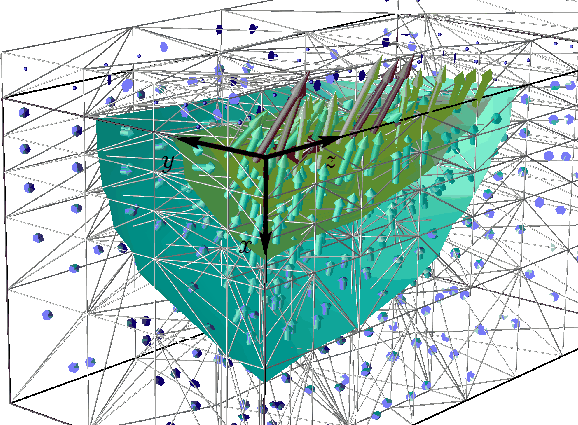Figure 4.7 shows the corresponding gradient field and iso-surfaces of the dopant concentration after a couple of refinement and error estimation cycles. As depicted in Table 4.1 it is possible that for one time step several refinement procedures are carried out. The gradient vectors are calculated for every tetrahedron using Equation (3.16). The orientation of the gradient points towards higher concentration values. The direction is perpendicular to the iso-surfaces of the dopant concentration. The gradient field varies much stronger along the $x$ - and the $y$ -direction of the open band, which forces a higher mesh density along these directions. The variation along the $z$ -direction is quite small and the granularity of the initial mesh should be kept.

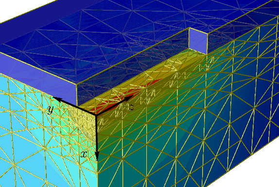
As shown in Figure 4.8 the refinement does not alter the edge length along the $z$ -direction of the cuboid, whereas along the short sides a much higher mesh density arises and the resolution for the diffusion calculation is increased. Other parts of the structure are completely untouched so that the overall number of mesh elements is kept fairly small which is important for the performance of the diffusion simulation.

Figure 4.8: Due to the combination of error estimation and anisotropic mesh refinement a good balance between the accuracy and the number of mesh elements was found. The refinement region is located in regions of high gradient field variations.