Subsections

• 6.4.1 Cubic Grid Based Meshes
• 6.4.2 Unstructured Tetrahedral Meshes
• 6.4.3 Resulting Unstructured k-Space Tessellation

6.4 k-Space Mesh Generation

Due to the high symmetry of the Brillouin zone, the discretization of the $\mathbf{k}$ -space domain can be reduced to the irreducible wedge, the properties of which are already discussed in Section 6.2. Several discretization methods based on different mesh generation regimes are proposed in literature [117]. One very common method for three-dimensional mesh generation is the so-called cubic grid method.

6.4.1 Cubic Grid Based Meshes

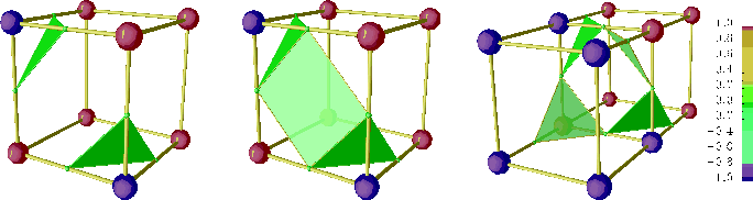
The basic idea behind this method is to subdivide the whole domain to be meshed into cubes of equal size. Different to an octree mesh approach the size of the cubes does not vary over the domain. The problem with cubic grids is that, if scalar data are stored on such grids in a 0 -face relation, the linear interpolation over the element becomes ambiguities. Figure 6.5 shows such inconsistent disambiguation for a particular constellation of scalar data stored related to the vertices. The linear interpolation is not well defined which causes different possible constellation of the shown iso-surface.

Figure 6.5: Inconsistent disambiguation. Different possible iso-surface representation for an ambiguous scalar data vertex relation shown in the left and in the middle. Inconsistent disambiguation between adjacent cubes causes a surface rupture, shown right.

To overcome these ambiguities the cubes are divided into tetrahedra, because on a tetrahedron the linear interpolation as described in Section 3.1.3 becomes unique and the iso-surfaces between two neighboring tetrahedra are conformal. Two methods are known for the tetrahedral decomposition which results in five or six tetrahedra per cube as seen in Figure 6.6(b) and Figure 6.6(e), respectively.

The decompositions of a cube into five tetrahedra yields an orientation switch of two opposite diagonal face edges of the cube. Due to this fact, the tessellation of one cube, as part of a larger cubic grid, forces a particular tessellation of all neighboring cubes to guarantee a conformal mesh. This means that, if such five-decompositions cubes are stacked together to a chain, the mesh of each cube must be rotated by an angle of $\pi/2$ .

For the tessellation of a cube into six tetrahedra, the orientations of opposite face edges are equal. This enables an independent partitioning under the assumption that every cube is fractionized by the same procedure and direction of the cuts. Non-conformal mesh constellations during the partitioning process vanish completely, if and only if every cube of the whole cubic grid is split by the same method.

Due to the special geometric property of the first octant of the Brillouin zone, a tessellation based on a cubic grid with a cube decomposition of five or six tetrahedra per cube is possible but based on the explanations above a decomposition into six tetrahedra is preferred and used in this work.

Figure 6.6: Decompositions of a cube into five tetrahedra (first row) and six tetrahedra (second row). The decomposition of the cube into six tetrahedra can be reached by an intermediate step, where the cube is split into two prisms. Each of the prisms is afterwards divided into three tetrahedra.

Figure 6.7: First octant of the silicon Brillouin zone. For the spatial discretization a cubic grid based tessellation scheme was used with constant grid spacing. The right part of the picture shows surfaces of constant energy for the first conduction band of silicon, the left part additionally holds mesh information. The wave vector is plotted in units of $2\pi /a_0$ .

Figure 6.7 shows the discretization of one octant of the Brillouin zone, based on a cubic grid approach with constant grid spacing. For the cube decomposition a six tetrahedra approach was chosen as shown in the second row of Figure 6.6.

The advantage of easy construction has as big counterbalance, the disadvantage that the mesh density is constant over the whole simulation domain. In [117] an algorithm is proposed which can deal with different mesh densities based on a so-called octree mesh approach, but the refinement zone is limited to a cuboidal region and therefore not very flexible. This gives rise to unstructured tetrahedral based meshes.

6.4.2 Unstructured Tetrahedral Meshes

State-of-the-art approaches as e.g. presented in [112] start with a simple decomposition of the irreducible wedge, which contains six vertices, into four tetrahedra. This initial mesh is divided into several tetrahedra by inserting new vertices on edges. A new vertex on an edge forces the division of a tetrahedron into two parts and therefore a finer mesh can be produced, cf. Section 2.2.2

One of the most flexible ways to generate unstructured meshes is to use a mesh generator which can produce meshes with different mesh densities in particular regions of the domain to be meshed. In this work DELINK [17] was used to generate the unstructured meshes for the demands of full band Monte Carlo simulations. The mesh was afterwards ``fine tuned'' by a recursive refinement procedure controlled by the scalar attribute stored on the mesh, which is discussed in detail in Section 6.4.3. Figure 6.8 shows the result of this meshing procedure for the first conduction band of silicon.

Figure 6.8: First octant of the silicon Brillouin zone. For the spatial discretization a pure unstructured tessellation scheme was used. The right part of the picture shows surfaces of constant energy for the first conduction band, the left part additionally holds mesh information. The wave vector is plotted in units of $2\pi /a_0$ .

6.4.3 Resulting Unstructured k-Space Tessellation

Figure 6.9: One quarter of $\{100\}$ -planes; Contours of constant energy for the first three conduction bands and the heavy hole band in silicon with additional mesh information are shown. The wave vector is plotted in units of $2\pi /a_0$ and the energy in $\MR{eV}$ with a band gap offset for silicon of $1.12 \MR{eV}$ for the valence band.

In the following a tetrahedron based mesh is used which enables calculation in the $\mathbf{k}$ -space domain in a simple and robust manner [118]. Flexible element grading allows to keep the total number of tetrahedra low and guarantees a good spatial resolution in regions of interests. These regions are mostly determined by an electron or hole distribution function that yields a higher population, which is important for full band Monte Carlo simulations. These domains should therefore be tracked very meticulously.

With respect to the complexity of the given band diagram different tessellations have been developed for the first, second, and the third conduction band and one mesh for the valence bands. 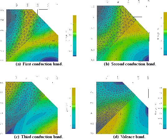Starting from an initial unstructured mesh which was produced with DELINK [17] a recursive tetrahedral bisection approach, as described in Section 2.2.3, was used to generate a finer mesh in different regions of the irreducible wedge, which is shown in Figure 6.9.

For the conduction band it is important to refine those regions of low energy values opposite to the mesh for holes where a finer mesh is set in regions of high energy values. So only those regions of interest have been refined with the recursive tetrahedral bisection method, other regions are left untouched.

Figures 6.9(a), Figure 6.9(b), and Figure 6.9(c) show constant energy contours and the resulting $\mathbf{k}$ -space mesh plots for the first, second, and third conduction band respectively. One can clearly observe a higher mesh density in regions of low energy values. Regions with high energy values are untouched by the recursive tetrahedral bisection refinement and show therefore the density of the initial mesh as produced with DELINK.

Since the valence bands show there maximum exact in the $\Gamma$ -point, only in this area a finer mesh is used. Opposite to the meshes for the first three valence bands, regions of low energy are untouched, so they show the mesh density of the initial mesh. The energy contour plot for the heavy hole band and the mesh plot for all hole bands is shown in Figure 6.9(d).

In the following three examples are presented, where the first deals with the calculation of density of states and the relation to analytical band structure approximations. The next example is focused on average kinetic energy calculations and the comparison of two different mesh approaches, namely the cubic grid approach and the unstructured mesh approach as presented in Section 6.4.1 and Section 6.4.2, respectively. The example section is closed by the electron velocity example which also deals with two different meshing approaches and the impact on the calculation of electron velocity.