3.5.4 Quantum Transmitting Boundary Method
An alternative method to solve the SCHRÖDINGER equation has been
proposed by FRENSLEY and EINSPRUCH [154]
which is based on the tight-binding quantum transmitting boundary method
(QTBM) introduced by LENT [155]. It has been used to
simulate electron transport in resonant tunneling diodes [153]. The
method is based on the finite-difference approximation of the stationary
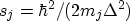
one-dimensional SCHRÖDINGER equation (3.61) on an equidistant
grid with an effective mass  and a grid spacing
 |
(3.84) |
where
 and
and
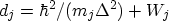 . For the evaluation of the transmission coefficient it is necessary to
assume open boundary conditions. They are introduced by writing the wave functions
at the boundaries of the simulation domain as
. For the evaluation of the transmission coefficient it is necessary to
assume open boundary conditions. They are introduced by writing the wave functions
at the boundaries of the simulation domain as
and relate them to the wave functions outside of the simulation domain by
This introduces four unknowns and two equations into the system.
Setting
eliminates the unknown values of  and
and
 and gives
a linear system for the
and gives
a linear system for the
 complex values
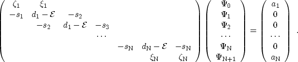 |
(3.91) |
Setting  and
and
 yields the values of the wave function in the
whole simulation domain for an incident wave from the left side like in the
transfer-matrix method. The method is easy to implement, fast, and more robust
than the transfer-matrix method. A further advantage of this method is its
suitability for two- and three-dimensional problems. It thus represents a much
more powerful method than the transfer-matrix based methods which are limited
to one-dimensional problems only. Note that the QTBM is closely linked with
the non-equilibrium GREEN's function formalism (NEGF, see Section 2.4.3.4): The
matrix in expression (3.91) is the inverse of the retarded
GREEN's function (2.25) for an open system without
scattering. However, the values of
yields the values of the wave function in the
whole simulation domain for an incident wave from the left side like in the
transfer-matrix method. The method is easy to implement, fast, and more robust
than the transfer-matrix method. A further advantage of this method is its
suitability for two- and three-dimensional problems. It thus represents a much
more powerful method than the transfer-matrix based methods which are limited
to one-dimensional problems only. Note that the QTBM is closely linked with
the non-equilibrium GREEN's function formalism (NEGF, see Section 2.4.3.4): The
matrix in expression (3.91) is the inverse of the retarded
GREEN's function (2.25) for an open system without
scattering. However, the values of  and
and  are complex, so the
matrix admits complex eigenvalues and complex solving routines are necessary.
are complex, so the
matrix admits complex eigenvalues and complex solving routines are necessary.
A. Gehring: Simulation of Tunneling in Semiconductor Devices