5.6.3.2 Calibration Task

The calibration of the TSUPREM-IV parameters as described above was performed with the combination of the simulated annealing and the gradient based optimization algorithm. Note that two measured points were ignored in this experiment since their given concentration is above the implanted dose. Table 5.1 depicts all parameters that were optimized during the calibration task.

Table 5.1: Parameters as they were used in the calibration of the clustering model, their ranges, and the found optimal value.

Variable	default value	minimum	maximum	optimum	unit
$\mathrm{D.0}$	$51.0$	$25.0$	$1000.0$	$694.335$	$cm^2s^-1$
$\mathrm{D.E}$	$1.77$	$1.4$	$1.85$	$1.5048$	$eV$
$\mathrm{CL.KFI.0}$	$5.0\cdot 10^{24}$	$1.0\cdot 10^{20}$	$1.0\cdot 10^{28}$	$6.3213\cdot 10^{26}$	$cm^{-3(1+\mathrm{isfi}-\mathrm{ifi})}s^-1$
$\mathrm{CL.KFI.E}$	$3.774$	$3.4$	$6.0$	$3.91624$	$eV$
$\mathrm{CL.KFC.0}$	$4.368\cdot 10^{19}$	$1.0\cdot 10^{17}$	$7.0\cdot 10^{19}$	$6.95285\cdot 10^{19}$	$cm^{-3(1+\mathrm{isfc}-\mathrm{ifc} -\mathrm{cf})}s^-1$
$\mathrm{CL.KFC.E}$	$4.95$	$4.9$	$5.2$	$4.90781$	$eV$
$\mathrm{CL.KR.0}$	$2.8\cdot 10^{16}$	$1.5\cdot 10^{16}$	$1.0\cdot 10^{18}$	$1.42833\cdot 10^{17}$	$cm^{-3(1-cr)}s^-1$
$\mathrm{CL.KR.E}$	$3.57$	$3.0$	$3.62$	$3.61939$	$eV$
$\mathrm{CL.KFCI}~(\alpha)$	$1100$	0	$5000$	$1336$	$1$
$\mathrm{CL.CR}$	$1.0$	$0.98$	$8.0$	$0.982801$	$1$
$\mathrm{CL.CF}$	$1.0$	$0.5$	$1.03$	$1.02736$	$1$

To account for the range of $\approx 3$ decades of the dopant concentration and under the assumption that all computed concentrations assume positive values $> 0$ the following scale function $S(p)$ was used to compute a deviation of a computed from a measured point:

$$S(p_m,p_c) = 100.0\cdot\left(10^{\ensuremath{\left\vert\frac{\log... ...ensuremath{\max\left[\log_{10}p_m, \log_{10}p_c\right]}}\right\vert}} -1\right)$$ (5.22)

where $p_m$ denotes a measured concentration and $p_c$ denotes a computed one (delivered by TSUPREM-IV). The error vector was then again computed according to (5.2). The obtained (optimized) parameter values are shown in Table 5.1.

Figure 5.28: Deviation of measured and computed cluster concentration (with the calibrated model). The reference dopings are drawn in thin lines.

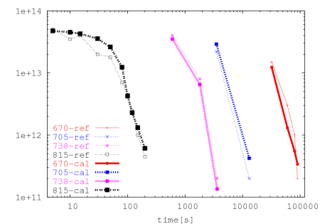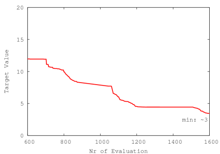
Fig. 5.28 depicts the resulting deviation of computed from measured dopings for the model parameters given in column "optimum" of Table 5.1. Fig. 5.29 and Fig. 5.30 depict the progress of the combined (simulated annealing and local) optimizer. The optimization started with a target value of $t_\mathrm{opt} = 1037$. The best target of $3.44$ was reached after $\approx 1600$ evaluations. The optimization was stopped after a total of $3300$ evaluations. No improvement in the target value was found for evaluation numbers $1600 - 3300$.

Figure 5.29: Progress of combined optimizer. The plot shows the first $1600$ evaluations. The optimizer started at a target value of $\approx 1050$.

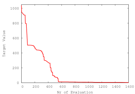Figure 5.30: This plot depicts a detailed view of Fig. 5.29. Evaluation numbers $600 - 1600$ are shown. The final optimum of $3.44$ was reached after $1600$ evaluation. No further improvement was found within another $1700$ evaluations.

2003-03-27