Genetic Optimizer

For our inverse modeling application we obtained the best results with the genetic optimizer with the STEADY-STATE algorithm, the ROULETTE-WHEEL selection scheme, and the one-point and the two-point crossover methods respectively. We used a replacement percentage of $0.7$ and a population size of $40$ ($28$ new individuals are introduced in every generation). Since GALIB does not directly support parallel target evaluation the optimizer takes care of evaluating several jobs in parallel.

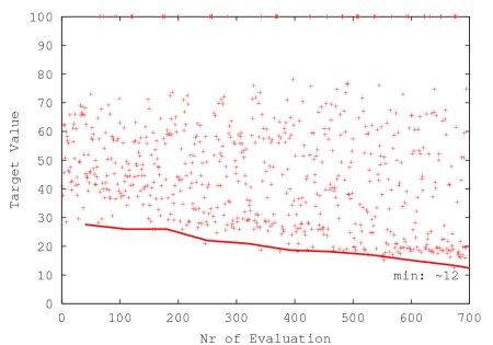
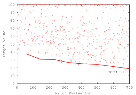
Several experiments with different crossover and mutation probabilities were carried out. Fig. 5.17 and Fig. 5.18 depict the evolution of the genetic algorithm for two different combinations of crossover and mutation probability and crossover method. The solid line is a plot of the best individual of each generation. Note that the best individual within a population sometimes occurs at a lower evaluation number thus appearing below the solid line. The parameter combination depicted in Fig. 5.17 leads to the best result for our application.

Figure 5.17: Evolution of the genetic optimizer for ${\ensuremath P_{\!cr\!oss}}{} = 0.9 \mathrm{,}\ \mathit{P_{mut}} = 0.2$,
and two-point-crossover.

Figure 5.18: Evolution of the genetic optimizer for ${\ensuremath P_{\!cr\!oss}}{} = 0.8 \mathrm{,}\ P_{mut} = 0.3$,
and one-point-crossover.

2003-03-27