5.6.2.3 Results

In the following several experiments carried out with the combination of very fast simulated re-annealing and a local optimization strategy are presented. The optimizations were performed with different numbers of initial evaluations and evaluations between two sub-optimization runs.

Fig. 5.24 depicts the case of a combined optimization

Figure: 5.24 Combination of very fast simulated re-annealing with a gradient-based optimizer. The very fast simulated re-annealing algorithm performed the first $70$ evaluations, the gradient-based optimizer evaluated the rest. The best target value from the very fast simulated re-annealing stand-alone run (blue dotted line) was reached after $\approx 300$ evaluations.

with $70$ initial evaluations. Only one sub-optimization task was performed, the optimization was stopped after the first return of the gradient-based optimizer. The blue dotted line in Fig. 5.24 depicts as a reference the evolution of the stand-alone very fast simulated re-annealing run (is identical with the red solid line of Fig. 5.19). Although the stand-alone run converges faster in the beginning, the target value of $8$ was already reached after $\approx 300$ evaluations. Additionally, the final target was improved to $\approx 7$.

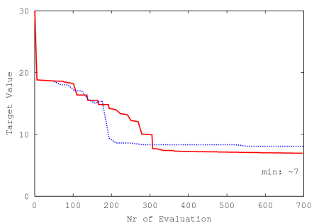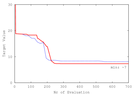
Fig. 5.25 depicts a strategy that reaches the best target of the reference run even faster. In this experiment the optimizers are used alternately. The best target of one optimizer is thereby taken as initial guess for the other optimizer respectively. An initial number of $100$ evaluations were performed before the sub-optimization task was initiated the first time. As soon as an improve in the target value was detected the sub-optimization task was terminated and the master continued with its best state updated to the result of the gradient-based optimizer. The interval between two sub-tasks was set to $30$.

Figure: 5.25 Better combination of of very fast simulated re-annealing and a gradient-based optimizer. The optimizers are started alternately. An initial number of $100$ evaluations was performed by the master, then the sub-optimization task was invoked after every $30$ evaluations. The sub-task was terminated as soon as the target was improved. With this strategy the target from the reference run was already reached after $\approx 230$ evaluations.

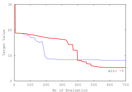
The strategy depicted in Fig. 5.26 results in the best target value for the given number of maximum evaluations ($700$) for all experiments that were carried during this comparison of optimization strategies. Here $70$ initial evaluations were performed and $40$ evaluations were performed between two consecutive sub-optimization runs.

Figure: 5.26 This combination of very fast simulated re-annealing and a gradient-based optimizer results in the best target value for the given maximum number of evaluations. An initial number of $70$ evaluations was performed. The interval between two sub-tasks was set to $40$.

2003-03-27