4.6.2 Time Evolution

The different material regions must be taken into account during time evolution, especially for the simulation of etching. Common approaches use a single velocity field which is set up in dependence of the material types on the surface [110]. This field is assumed to be constant for the duration of the time integration step. However, if the etch front reaches another material within that time step, for which the value of the etch rate differs significantly, as is the case for mask or etch stop layers, the surface is advanced with the wrong velocity. For the LS representation introduced in (4.19) a more accurate technique is presented in this section, which is able to resolve varying surface velocities with sub-time-step accuracy.

Initially only the topmost LS function ${\Phi}_{M}$ , which represents the surface, is updated in time. Thereby, the surface velocities of different materials which are on the surface and which can be retrieved from the surface material function (4.20) are incorporated. In the following, it is always assumed that material of type ${\mathcal{M}}_{M}$ is deposited, if the surface velocities are positive. If another material should be deposited instead, a new material layer must be added, as described previously. Negative surface velocities stand for material removal, and the material dependence on the surface velocity must be incorporated during the time evolution of ${\Phi}_{M}$ .

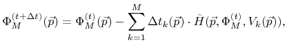
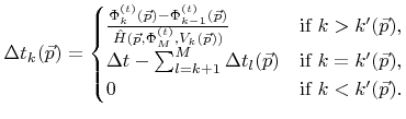
After updating the topmost LS function ${\Phi}_{M}$ in time, all other LS functions representing the interfaces between material regions, are adapted according to the Boolean operation

$${\Phi}_k^{({t}+\Delta{t})}({\vec{x}})=\max\left({\Phi}_k^{({t})}({\vec{x}}),{\Phi}_{M}^{({t}+\Delta{t})}({\vec{x}})\right).$$ (4.22)

This adaption rule maintains relation (4.21). For pure deposition processes, where the surface velocity is positive everywhere on the surface, (4.22) does not change the other LS functions. However, if there are any regions on the surface with negative surface velocities, these Boolean operations must be performed.

There is still the open question of how to change ${\Phi}_{M}$ under consideration of the different material regions with sub-time-step accuracy. For simplicity ${M}$ different velocity fields ${V}_k({\vec{x}})$ $(1\leq k \leq {M})$ are introduced, one for each material type. The value of ${V}_k({\vec{x}})$ at a certain surface point ${\vec{x}}\in{\mathcal{S}}$ is defined as the surface velocity, which would be obtained, if material ${\mathcal{M}}_k$ was on the surface at that point, i.e. $\funcmat ({\vec{x}})=k$ holds. However, ${V}_k({\vec{x}})$ is still calculated using the arriving flux distribution ${\Gamma}({\vec{x}};{q},{\vec{\omega}}, {E})$ . This distribution can be assumed to be constant for the duration of the time integration step, because small changes of the geometry usually do not show much influence on particle transport. Even if the material type changes on small parts of the surface during the time step, which leads to different reemission probabilities, the flux distribution remains approximately the same.

Due to the convention that only the topmost material ${\mathcal{M}}_{M}$ can be deposited, the surface velocity fields must obey

$${V}_k({\vec{x}}) \in \mathbb{R}^{-}_0 \ 1\leq k < {M},$$ (4.23)

$${V}_{M}({\vec{x}}) \in \mathbb{R}.$$ (4.24)

The time evolution of ${\Phi}_{M}$ is computed using a generalization of the update rule (3.5)

$${\Phi}_{M}^{({t}+\Delta {t})}({\vec{p}})={\Phi}_{M}^{({t})}({\vec... ...t}_k({\vec{p}}) \cdot {\hat{H}}({\vec{p}},{\Phi}_{M}^{({t})},{V}_k({\vec{p}})),$$ (4.25)

which is applied to all active grid points ${\vec{p}}\in{\mathcal{L}}_0^{({t},{M})}$ . Here, in accordance with the sparse field method, ${\mathcal{L}}_0^{({t},{M})}$ denotes the active layer of ${\Phi}_{M}$ at time ${t}$ . $\Delta {t}_k({\vec{p}})$ denotes the time for which the surface velocity ${V}_k({\vec{p}})$ is used during the time integration of the LS value at point ${\vec{p}}$ . The sum of all these times must satisfy $\sum_{k=1}^{M}\Delta{t}_k({{\vec{p}}})=\Delta{t}$ . To incorporate material-dependent surface velocities with sub-time-step accuracy they are approximated for a given time step $\Delta{t}$ using

$$\Delta {t}_k({{\vec{p}}}) = \begin{cases}\frac{{\Phi}_k^{({t})}({... ... & \text{if} \ k=k'({\vec{p}}), \\ 0 & \text{if} \ k<k'({\vec{p}}). \end{cases}$$ (4.26)

For each active grid point ${\vec{p}}$ the material number $k'({\vec{p}})$ is chosen to be the smallest number $(1\leq k'({\vec{p}}) \leq {M})$ for which all $\Delta {t}_k({\vec{p}})$ are non-negative, if they are calculated according to (4.26). If ${V}_{M}({\vec{p}})$ is positive, $k'({\vec{p}})$ is always set to ${M}$ . $k'({\vec{p}})$ can be interpreted as the material type which is locally on the surface after the time integration step. Insertion of (4.26) into (4.25) yields

$${\Phi}_{M}^{({t}+\Delta {t})}({\vec{p}}) = {\Phi}_{k'}^{({t})}({\... ...}({\vec{p}}) \cdot {\hat{H}}({\vec{p}},{\Phi}_{M}^{({t})},{V}_{k'}({\vec{p}})).$$ (4.27)

It should be noted that it is not necessary to evaluate the velocity fields ${V}_k$ for all $k$ and at all active grid points ${\vec{p}}\in{\mathcal{L}}_0^{({t},{M})}$ . For an active grid point ${\vec{p}}$ it is sufficient to calculate ${V}_k({\vec{p}})$ for $k'({\vec{p}})\leq k\leq {M}$ . ${V}_k({\vec{p}})$ with $k<{M}$ is also not relevant, if ${\Phi}_k^{({t})}({\vec{p}})={\Phi}_{k-1}^{({t})}({\vec{p}})$ . Moreover, if ${V}_{M}({\vec{x}})$ is never positive, due to the applied model, then the determination of ${V}_{M}({\vec{p}})$ can also be omitted in the case of ${\Phi}_{M}^{({t})}({\vec{p}})={\Phi}_{{M}-1}^{({t})}({\vec{p}})$ . Hence, for a certain active grid point only the local surface velocities for those materials, which are actually involved during the time step, must be determined.

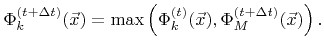
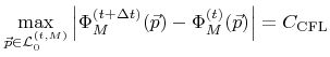
The time integration step $\Delta{t}$ is chosen according to (3.32) in such a way that

$$\max_{{\vec{p}}\in {\mathcal{L}}_0^{({t},{M})}}\left\vert{\Phi}_{... ...elta {t})}({\vec{p}})-{\Phi}_{M}^{({t})}({\vec{p}})\right\vert = {C_\text{CFL}}$$ (4.28)

is satisfied. Due to the limitation ${C_\text{CFL}}\leq\frac{1}{2}$ (4.8) it is sufficient for the solution of (4.26) to store only LS values up to an absolute value of $1$ within the H-RLE data structures for the LS functions ${\Phi}_1,{\Phi}_2,\ldots,{\Phi}_{{M}-1}$ . LS values of positive and negative undefined grid points are again considered to be equal to $+\infty$ and $-\infty$ , respectively (compare Section 4.2.1).

The presented multi-LS method can be realized by adapting the time integration procedure described in Section 4.3.1. While iterating over the surface LS function ${\Phi}_{M}$ using a stencil of iterators, which allows the calculation of the required finite differences, ${M}-1$ additional basic iterators are simultaneously moved over the corresponding H-RLE data structures of ${\Phi}_1,{\Phi}_2,\ldots,{\Phi}_{{M}-1}$ . These iterators allow access to the LS values as needed in (4.26).