4.7 Directional Visibility Check

Some processes are characterized by almost unidirectional and normal incident particle transport from the source plane to the surface. In this case the H-RLE data structure can be useful for the computation of surface velocities for the active grid points. The surface velocity field at active grid points is usually obtained by taking the surface velocity of the closest surface point. The surface velocity of a surface point depends on the visibility from the particle source along the incidence direction. Instead of determining the visibilities for surface points and mapping the information to the active grid points, it is possible to compute the visibility information directly for all active grid points.

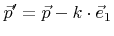
In the following section, an active grid point is called visible, if the corresponding closest surface point is visible. Furthermore, it is assumed that the incidence direction is equal to the positive ${x}_1$ -direction. Then, an active grid point ${\vec{p}}$ can be regarded as visible, if the LS values of all grid points ${\vec{p}}'={\vec{p}}-k\cdot{\vec{e}}_1$ with $k>0$ are larger than or equal to that of grid point ${\vec{p}}$

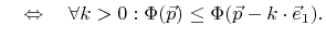$${\vec{p}}\ \quad \Leftrightarrow \quad \forall k>0: {\Phi}({\vec{p}}) \leq {\Phi}({\vec{p}}-k\cdot{\vec{e}}_1).$$ (4.29)

Thereby, the LS values of positive and negative undefined grid points are again assumed to be $\pm\infty$ , respectively. Figure 4.13 illustrates by means of an example, which active grid points are visible. Taking advantage of the lexicographical ordering, it is sufficient to iterate once over the H-RLE data structure to determine the visibilities for all active grid points. Hence, this visibility test is of optimal complexity ${\mathcal{O}}({{N}_\text{D}})$ , where ${{N}_\text{D}}$ denotes again the number of defined grid points, which is proportional to the surface size measured in grid spacings.

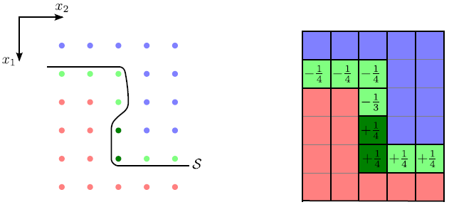
Figure 4.13: A surface ${\mathcal {S}}$ and its H-RLE representation are shown. In this example, the LS values are only defined for the active grid points. Positive (blue) and negative (red) runs of undefined grid points are assumed to have LS values $+\infty$ and $-\infty$ , respectively. The dark green grid points do not fulfill the visibility criterion.