4.7.1 Directional Etching

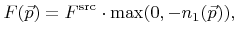
For a visible grid point the local flux on the surface can be computed as

$${F}({\vec{p}})={F}^{\text{src}}\cdot\max(0, -{n}_1({\vec{p}})),$$ (4.30)

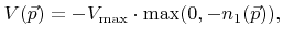
where ${F}^{\text{src}}$ denotes the incident flux from the source. ${n}_1$ is the first component of the normal vector ${\vec{n}}$ as defined in Section 3.3.1. If the etch yield is independent of the incidence direction, the surface velocity can simply be set proportional to the total flux. Therefore the surface velocity can be written as

$${V}({\vec{p}})=-{V}_{\text{max}}\cdot\max(0, -{n}_1({\vec{p}})),$$ (4.31)

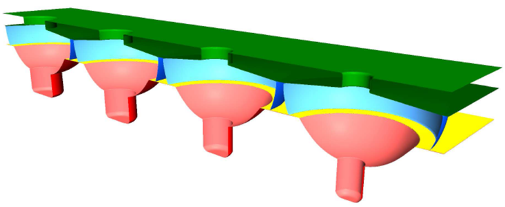
where ${V}_{\text{max}}$ is the maximum etch rate for normal incidence. As a demonstration, directional etching is applied to the structure given in Figure 4.12. The result, after a process time of 60 time units, is shown in Figure 4.14. The maximum etch rate was assumed to depend on the material. 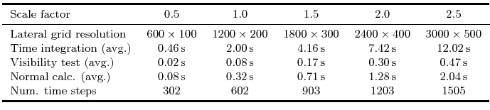${V}_{\text{max}}=\num{0.025}$ and ${V}_{\text{max}}=1$ (grid spacings per time unit) were assumed for the mask ( ${\mathcal {M}}_3$ ) and the substrate ( ${\mathcal {M}}_1$ ), respectively. The average computation times for time integration, normal calculation, and directional visibility check are given in Table 4.2 and prove the linear scaling with surface size.

The rounding at the bottom observed in Figure 4.14 can be ascribed to the finite difference scheme for solving the LS equation. All schemes inherently introduce some amount of dissipation in order to obtain a stable solution. The rounding can be reduced, if a finer grid with a smaller grid spacing is used for the calculation.

Figure 4.14: The structure given in Figure 4.12 after processing with a directional material-dependent etch process.

Table 4.2: The average computation times for a time integration step, the directional visibility test, and the normal vector calculation for the directional etching process shown in Figure 4.14.

$\parbox{\textwidth}{ \small \begin{tabular}{lccccc} \toprule {Scale ... ...}$\ & $\num{903}$\ & $\num{1203}$\ & $\num{1505}$\\ \bottomrule \end{tabular}}$