5.2.2 Tangential Disks

The LS method requires a surface velocity field which is commonly obtained by extrapolating the velocities computed on the surface (compare Section 3.2.4). If the active grid points are very close to the surface, which is the case for the sparse field method, it is possible to calculate the surface rates directly for those grid points [112,A13]. In this way the extrapolation procedure can be avoided and no extra memory is needed to store the velocities for the discretized surface.

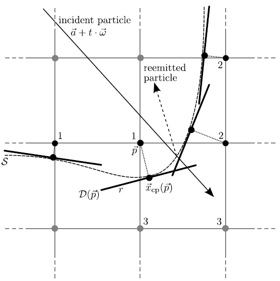
As proposed in [A16,A20] tangential disks ${\mathcal{D}}({\vec{p}})$ can be defined for all points on the surface, which are closest to any active grid points ${\vec{p}}\in{\mathcal{L}}_0$ . Hence, for each active grid point ${\vec{p}}$ a disk is defined which serves as a neighborhood for its corresponding closest surface point ${\vec{x}}_{\text{cp}}({\vec{p}})$ . The closest surface point ${\vec{x}}_{\text{cp}}({\vec{p}})$ , which is also the midpoint of the tangential disk ${\mathcal{D}}({\vec{p}})$ , is approximated using (3.23). The orientation of the disk is given by the surface normal which is approximated by ${\vec{n}}({\vec{p}})$ as defined in (3.22). Hence, the tangential disk ${\mathcal{D}}({\vec{p}})$ is described by

$${\mathcal{D}}({\vec{p}}) = \lbrace {\vec{x}} : \lVert{\vec{x}}-{\... ...{x}}-{\vec{x}}_{\text{cp}}({\vec{p}})\right)\cdot{\vec{n}}({\vec{p}})=0 \rbrace$$ (5.18)

with ${r}$ denoting the radius. Disks have the advantage that intersection tests with rays are relatively simple. A ray with parameterization ${\vec{x}}(t)={\vec{a}}+t\cdot{\vec{\omega}}$ strikes the disk ${\mathcal{D}}({\vec{p}})$ on the front side, if the following condition is fulfilled

$$\cos{\theta}>0 \quad \wedge \quad \lVert{\vec{x}}_{\text{rel}}\cd... ...}}({\vec{p}})\cdot{\vec{x}}_{\text{rel}}\right)\rVert \leq {r}\cdot\cos{\theta}$$ (5.19)

with $\cos{\theta}:=-{\vec{\omega}}\cdot{\vec{n}}({\vec{p}})$ and ${\vec{x}}_{\text{rel}}:={\vec{a}}-{\vec{x}}_{\text{cp}}({\vec{p}})$ . In this case the corresponding particle contributes to the rates of grid point ${\vec{p}}$ according to (5.15). To calculate the surface rates correctly for active grid points, whose corresponding tangential disks are partially behind the surface ${\mathcal {S}}$ due to the curvature, it is necessary to prolong the calculation of the particle trajectory for a few grid spacings from the surface intersection point (see Figure 5.1). However, the first intersection point with the surface is stored and used as a starting point for reemitted particles.

Figure: 5.1 If a particle trajectory intersects any tangential disk (thick black) ${\mathcal{D}}({\vec{p}})$ , it contributes to the rates of the corresponding active grid point (black) ${\vec{p}}\in{\mathcal{L}}_0$ . Due to the curvature of the surface ${\mathcal {S}}$ , the calculation of the particle trajectory must be continued for a few grid spacings in order to obtain correct rates. However, new reemitted particles (dashed) are always launched from the surface intersection point. To avoid multiple intersection tests of the same disk, only those grid points which are opposite to the entry face are checked, if they are active and if their corresponding disk is intersected. The numbers show which points are processed in which cell.

The area of the disks is ${A}_{\text{ref}}=\pi{r}^2$ or in case of two dimensions, where the disks correspond to tangential segments, ${A}_{\text{ref}}=2{r}$ . Hence, the choice of the disk radius influences the statistical accuracy. Larger radii give better statistics at the expense of the spatial resolution which should be of same magnitude as the resolution of the surface. Hence the disk radius should be in the order of the grid spacing which was assumed to be unity.

In [A20] an upper limit for the radius was suggested. Within the sparse field method $\left\vert{\Phi}({\vec{p}})\right\vert\leq\frac{1}{2}$ holds for all active grid points. Furthermore, the approximation for the gradient is almost always larger than 1, thus $\lVert\nabla{\Phi}({\vec{p}})\rVert\geq1$ . This gives an upper limit for the distance to the approximated closest surface point $\lVert{\vec{p}}-{\vec{x}}_{\text{cp}}({\vec{p}})\rVert\leq\frac{1}{2}$ according to (3.23). If the radius is chosen in such a manner that

$${r}\leq\sqrt{1-\left(\textstyle\frac{1}{2}\right)^2}\approx\num{0.866},$$ (5.20)

the disk ${\mathcal{D}}({\vec{p}})$ is within the $2^{D}$ grid cells which are adjacent to the active grid point ${\vec{p}}$ . In very rare cases, when $\lVert\nabla{\Phi}({\vec{p}})\rVert\geq1$ is not fulfilled, it might be necessary to translate the disk towards ${\vec{p}}$ , in order to fit it into the surrounding cells. Much smaller disk radii than the given upper limit lead to worse statistics without improving the spatial resolution. 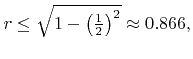Therefore, it is recommended to use a disk radius of 0.8 grid spacings [A20].

This way the computational effort for ray-disk intersection tests is minimized. Within a grid cell only the $2^{D}$ corner grid points have to be checked, if they are active, and if their corresponding tangential disks ${\mathcal{D}}({\vec{p}})$ are intersected. Hence, the same data structure can be used as the one needed for the multi-linear interpolation for the surface intersection test, which requires links to all its corners in order to access the corresponding LS values.