5.2.6 Spatial Subdivision

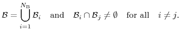
The cell-by-cell traversal to find intersections with the surface and the disks requires the determination of the face, through which a particle leaves a grid cell, in order to obtain the next cell. Intersections are only possible within grid cells which contain parts of the surface or parts of any disk. All other empty grid cells do not need to be tested for any kind of intersection. Therefore, it is possible to combine these empty grid cells to obtain larger boxes to be traversed simultaneously. In this way, if efficient data structures are used, which allow a fast determination of neighboring boxes, the computation time can be reduced. The goal is to find an appropriate decomposition of the simulation domain into a set of disjoint rectangular axis aligned subboxes ${\mathcal{B}}_1, {\mathcal{B}}_2,\ldots,{\mathcal{B}}_{{N}_{\text{B}}}$ :

$${\mathcal{B}} = \bigcup_{i=1}^{{{N}_{\text{B}}}} {\mathcal{B}}_i ... ...thcal{B}}_i\cap{\mathcal{B}}_j\neq\emptyset \quad \text{for all} \quad i\neq j.$$ (5.21)

Here ${\mathcal{B}}$ denotes the bounding box of the simulation domain. Binary space partition is commonly used to obtain a suitable decomposition [10,39]. Subsequent splitting of the domain at certain grid planes, until each non-empty cell is a subbox of its own, leads to an appropriate decomposition. Different strategies have been developed to choose the splitting planes and will be discussed later. The decomposition is usually stored using a kd-tree [39,134]. For each node at least the splitting plane and links to its two child nodes have to be stored. Each leaf corresponds to a subbox of the final decomposition.

Once the face through which a particle leaves a box is known, the next neighbor box can be accessed using the kd-tree. This requires an up traversal to the node which joins the branches of the corresponding leaves representing the current and the neighboring box. Then a down traversal is necessary, until the leaf node, which represents the neighboring subbox, is reached [10]. However, traversing upwards is only possible, if either the history of traversed nodes has been stored during down traversal, or, if links are available which give direct access to parent nodes.

The first approach is not very suitable for the previously presented rate calculation algorithm. Reemitted particles, which are launched from the surface intersection point, are buffered in a stack, while the trajectory of the incident particle is continued for a couple of grid spacings in order to consider potential disk intersections behind the surface. If only the initial position, which is the surface intersection, is stored with the new particles, the corresponding subbox must be re-determined before starting the trajectory calculation. To avoid the required costly complete top-down traversal, a reference to the subbox can be stored together with the position coordinates. Without parent links, the entire down traversal history would also have to be stored, which would slow down the entire simulation.

In the worst case a neighbor access within the kd-tree is of logarithmic complexity ${\mathcal{O}}(\log {{N}_{\text{B}}})$ . However, the neighbor box can be retrieved in constant time on average. Therefore the computational effort primarily scales with the average number of traversed subboxes.