2.4 Nonradiative Multi-Phonon Theory
For the level shift, it has been implicitly presumed that vibronic
transitions always take place at equilibrium configurations of the
defects. Thereby, it has been ruled out that the defects are thermally
excited
up to the intersection points of their adiabatic potentials (see Fig. 2.4). However,
this case has been accounted for in the nonradiative multi-phonon theory
(NMP) [107, 115]. This mechanism has already been suggested for random
telegraph noise and  noise in microelectronic devices [56], where only a
simplified description of NMP process has been employed. Furthermore, it is
also encountered in the context of phonon-assisted tunneling ionization of
deep centers [116, 117, 118] and discussed on various levels of theoretical
sophistication [119, 120, 55, 121, 122] including additional second-order
effects, such as the Coulomb energy [123, 124, 125] and field-enhancement
factors [116, 117].
noise in microelectronic devices [56], where only a
simplified description of NMP process has been employed. Furthermore, it is
also encountered in the context of phonon-assisted tunneling ionization of
deep centers [116, 117, 118] and discussed on various levels of theoretical
sophistication [119, 120, 55, 121, 122] including additional second-order
effects, such as the Coulomb energy [123, 124, 125] and field-enhancement
factors [116, 117].
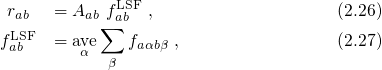
In NMP theory, the equation (2.21) is generalized to account for all possible thermal
excitations. Then the equation (2.21) must be rewritten as
where  is referred to as the lineshape function. ‘
 ’ denotes the thermal
average over all initial vibrational states
’ denotes the thermal
average over all initial vibrational states  and accounts for the thermal
excitations using a sum over weighted Boltzmann factors. The lineshape
function eventually depends on the Franck-Condon factor and thus on the
complicated shape of the adiabatic potentials of the defects. It is noted that these
potentials are not assessable via experiments but can also not be calculated using
first-principles calculations (see Section 3.3), which would by far exceed the current
computational capabilities. However, they can be reasonably approximated using the
harmonic approximation when only small displacements from the equilibrium
configuration of the defects are considered. In this approximation, the adiabatic
potentials are represented as a Taylor expansion whose linear term vanishes
close to the equilibrium configuration. As a result, these potentials become
parabolic and therefore, describe harmonic oscillators frequently used in solid
state physics. A corresponding configuration coordinate diagram for the
vibronic transitions of a defect is depicted in Fig. 2.4. The total energies
and accounts for the thermal
excitations using a sum over weighted Boltzmann factors. The lineshape
function eventually depends on the Franck-Condon factor and thus on the
complicated shape of the adiabatic potentials of the defects. It is noted that these
potentials are not assessable via experiments but can also not be calculated using
first-principles calculations (see Section 3.3), which would by far exceed the current
computational capabilities. However, they can be reasonably approximated using the
harmonic approximation when only small displacements from the equilibrium
configuration of the defects are considered. In this approximation, the adiabatic
potentials are represented as a Taylor expansion whose linear term vanishes
close to the equilibrium configuration. As a result, these potentials become
parabolic and therefore, describe harmonic oscillators frequently used in solid
state physics. A corresponding configuration coordinate diagram for the
vibronic transitions of a defect is depicted in Fig. 2.4. The total energies
 and
and  in Fig. 2.4 include the contributions from the defect
atoms along with its immediate surrounding (and the channel region) and
therefore correspond to the adiabatic potentials
in Fig. 2.4 include the contributions from the defect
atoms along with its immediate surrounding (and the channel region) and
therefore correspond to the adiabatic potentials  . For this
reason, their corresponding adiabatic potentials differ only in the location of
electron involved in the trapping process. In the case of
. For this
reason, their corresponding adiabatic potentials differ only in the location of
electron involved in the trapping process. In the case of  , the electron
resides in the channel while, for
, the electron
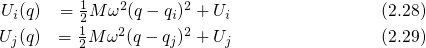
resides in the channel while, for  , it is located at the defect site. In
the harmonic approximation, the adiabatic potentials can be written as:
, it is located at the defect site. In
the harmonic approximation, the adiabatic potentials can be written as:
 stands for the vibrational frequency of the oscillator and determines the curvature
of the parabola while
stands for the vibrational frequency of the oscillator and determines the curvature
of the parabola while  is the mass of the oscillator. Analogously to the previous
section, the classical vibronic transitions are assumed to occur at the intersection
points of the adiabatic potentials. Therefore, the defect system must be thermally
excited from its initial configuration
is the mass of the oscillator. Analogously to the previous
section, the classical vibronic transitions are assumed to occur at the intersection
points of the adiabatic potentials. Therefore, the defect system must be thermally
excited from its initial configuration  to the intersection point IP
of the two parabolas in Fig. 2.4. At this point, the total energies
to the intersection point IP
of the two parabolas in Fig. 2.4. At this point, the total energies  and
and  equal and allow for an elastic tunneling transition. From there,
the system relaxes to the equilibrium configuration
equal and allow for an elastic tunneling transition. From there,
the system relaxes to the equilibrium configuration  with the energy
 . The energy difference between
  and
and  can be expressed as
 is the so-called thermodynamic trap level. It is given
relative to the conduction or the valence band edge for electron or hole
trapping
and determines the occupancy of the defect in thermal equilibrium. As demonstrated
in Fig. 2.4, the Huang-Rhys factor
is the so-called thermodynamic trap level. It is given
relative to the conduction or the valence band edge for electron or hole
trapping
and determines the occupancy of the defect in thermal equilibrium. As demonstrated
in Fig. 2.4, the Huang-Rhys factor  is defined by the energy differences
 and
and  , which are both equivalent to
  phonons
with an energy of
phonons
with an energy of  . That is, this quantity determines the intersection point of the
parabolas and eventually impacts the probability for an electron transition between
the defect and the channel. In the above NMP concept, it has been assumed that the
charge state of the defect does not affect the curvatures of
. That is, this quantity determines the intersection point of the
parabolas and eventually impacts the probability for an electron transition between
the defect and the channel. In the above NMP concept, it has been assumed that the
charge state of the defect does not affect the curvatures of  and
and  .
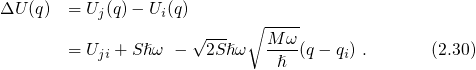
As a result, only a linear term in
.
As a result, only a linear term in  appears in equation (2.30). Note that
its sign is determined by the relative positions of
appears in equation (2.30). Note that
its sign is determined by the relative positions of  and
and  but has no
physical meaning. The forward and reverse barrier of this process are given by
and respectively.
but has no
physical meaning. The forward and reverse barrier of this process are given by
and respectively.
The NMP mechanism was suggested several decades ago but has been disregarded in
the context of NBTI so far. Nevertheless, this mechanism should be considered as a
possible description of charge trapping in NBTI. The underlying theory relies on the
complicated quantization effects of the nuclei system and is therefore quite
complex in its original variant. However, several convenient and accurate
approximations, including the version presented in this section, have been
developed over the years and allow for theoretical investigations on a device
level.
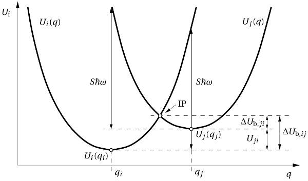
 and
and  show the adiabatic potentials for the case that
the electron is located in the channel or the defect, respectively. IP labels the
intersection point of
show the adiabatic potentials for the case that
the electron is located in the channel or the defect, respectively. IP labels the
intersection point of  and
and  , where the NMP process takes place in
the classical approximation. The electron capture or emission rates are primarily
determined by the NMP barriers
, where the NMP process takes place in
the classical approximation. The electron capture or emission rates are primarily
determined by the NMP barriers  and
and  , respectively.