or
or  between the intersection point of the parabolic potentials and its initial
ground state. For linear electron-phonon coupling, i.e.
between the intersection point of the parabolic potentials and its initial
ground state. For linear electron-phonon coupling, i.e.  , these
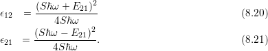
forward and reverse barrier energies are derived in Appendix D.2 to be
, these
forward and reverse barrier energies are derived in Appendix D.2 to be
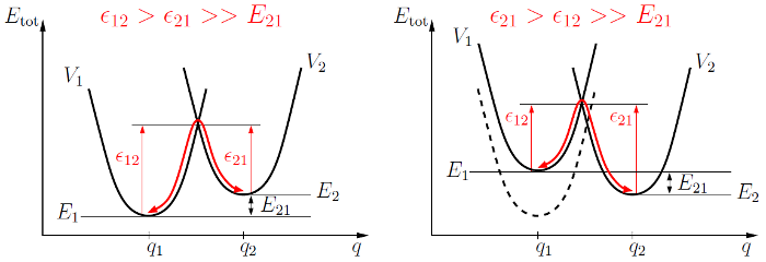
An alternative process excludes the absorption and emission of a photon, which is
actually the use condition of a MOSFET. This makes it a non-radiative
transition (NMP) [161, 111, 162, 130], like depicted in the right of Fig. 8.6. In a
classical transition the defect can only surmount the barrier or
between the intersection point of the parabolic potentials and its initial
ground state. For linear electron-phonon coupling, i.e. , these
forward and reverse barrier energies are derived in Appendix D.2 to be
When shifting the defect level by applying a bias, the defect system in state
 is shifted with respect to the defect system in state
  . Since the intersection
point is changed hereby, the transition rates are directly affected. This approach
was already used for the permanent component of the two-stage model depicted
in Fig. 8.5 and is schematically shown in Fig. 8.7 for two different bias
conditions.
. Since the intersection
point is changed hereby, the transition rates are directly affected. This approach
was already used for the permanent component of the two-stage model depicted
in Fig. 8.5 and is schematically shown in Fig. 8.7 for two different bias
conditions.
 as a function of the reaction coordinate
 for non-radiative multi-phonon emission assuming strong (
 )
and linear coupling (
)
and linear coupling ( ). Left: Without applied bias
  and
state
and
state  is preferred due to its lower total energy. Right: Applying a
bias induces an oxide electric field which shifts the defect state
is preferred due to its lower total energy. Right: Applying a
bias induces an oxide electric field which shifts the defect state  with
respect to state
with
respect to state  . At the same time the intersection point is changed and
consequently the barriers
. At the same time the intersection point is changed and
consequently the barriers  and
and  . For the case shown here the barriers
were changed by
. For the case shown here the barriers
were changed by  , i.e.
  , making the state
  more likely to
be occupied.
more likely to
be occupied.
When comparing Fig. 8.6 (right) with Fig. 8.7 (left), a strong difference in
 can be observed. While for small
  the relaxation energy
  is much smaller compared to
  , it is exactly the opposite for large
  .
Depending on which case to deal with, (8.20) and (8.21) can be further
approximated. In the first case this yields
.
Depending on which case to deal with, (8.20) and (8.21) can be further
approximated. In the first case this yields
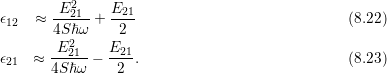
 , even quadratically, and not as much on the phonon part contained
in the relaxation energy, this case is called weak coupling. Usually one
deals with the other case, termed strong coupling, where the barriers are
The barriers here are dominated by the relaxation energy and only linearly
depend on
, even quadratically, and not as much on the phonon part contained
in the relaxation energy, this case is called weak coupling. Usually one
deals with the other case, termed strong coupling, where the barriers are
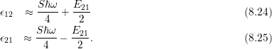
The barriers here are dominated by the relaxation energy and only linearly
depend on  . This approximation is also visible in Fig. 8.6 (right) for weak
and in Fig. 8.7 (left) for strong coupling. When comparing the barriers (8.24)
and (8.25) with those within the SRH model (8.13) and (8.14), it can be seen
that it is no longer necessary to distinguish whether the trap level is
below or above the reservoir level. Furthermore, in the NMP model both
barriers of the capture and emission process (
. This approximation is also visible in Fig. 8.6 (right) for weak
and in Fig. 8.7 (left) for strong coupling. When comparing the barriers (8.24)
and (8.25) with those within the SRH model (8.13) and (8.14), it can be seen
that it is no longer necessary to distinguish whether the trap level is
below or above the reservoir level. Furthermore, in the NMP model both
barriers of the capture and emission process ( and
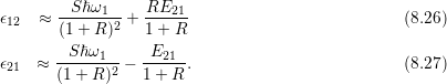
and  ) depend on
the applied field to the same degree with only opposite sign, as can be
easily seen in Fig. 8.7. As such the same amount one barrier is lowered is
added to the reverse barrier. The resulting field depence of
) depend on
the applied field to the same degree with only opposite sign, as can be
easily seen in Fig. 8.7. As such the same amount one barrier is lowered is
added to the reverse barrier. The resulting field depence of  and
and  is hence symmetric for linear coupling. By considering also quadratic
electron-phonon coupling terms [163, 111], this symmetry is lifted so that
one barrier is increased at the expense of the reverse barrier after [130]
with
is hence symmetric for linear coupling. By considering also quadratic
electron-phonon coupling terms [163, 111], this symmetry is lifted so that
one barrier is increased at the expense of the reverse barrier after [130]
with  as
as  . Unfortunately, this does not solve the undesired correlation
of
. Unfortunately, this does not solve the undesired correlation
of  and
and  , stated at the end of Chapter 8.1.