Subsections

• 8.3.1 The Equations
• 8.3.2 Transformation into the GSSE 
• 8.3.3 Results

8.3 Diffusion Simulation

The accurate simulation of the dopant atoms and their spatial distribution within devices is an important issue in modern TCAD. The characteristics of the manufactured device is determined by these issues, e.g., if devices rely on very shallow junctions to minimize the so-called short-channel effects [152]. Diffusion does not only occur in place of the introduction of dopant atoms, the so-called ion-implantation step, but also to electrically activate the implanted atoms. A comprehensive study of currently developed diffusion simulation methods is given in [69]. The simulations given here use the finite volume discretization method with very basic models to document the potential of GSSE as a mathematical framework for generic parabolic PDEs. The transformation of the given equations into executable C++ code and the corresponding alternative time discretization steps are the main parts, whereas the results show the feasibility.

8.3.1 The Equations

This example introduces a parabolic type of a PDE. As introduced in Section 2.1, time can be modeled by different numerical approximations. Here, an implicit and an explicit method are presented [67]. The following differential equation is used to describe a generic parabolic PDE, e.g., a diffusion process with boundary conditions:

$$\mathrm{div} \left( u \right) + \alpha \partial_t u = 0 \quad \textnormal{on} {\ensuremath{\Omega}}$$ (8.5)

$$\partial_n u = 0 \quad \textnormal{on}  {\ensuremath{\Gamma}}_1$$ (8.6)

$$u = f(x, y, z) \quad \textnormal{on}  {\ensuremath{\Gamma}}_2$$ (8.7)

By the use of the concepts presented the discretized formulation by the finite volume method is rendered similar to a generic elliptic equation, extended by an additional time derivative

$$\mathcal{L}_\mathrm{p\_fvm} (\mathrm{u})\equiv \sum_{v\rightarrow... ...) \frac{A}{d} + \frac{\mathrm{u} - \mathrm{u}_{\mathrm{old}}}{\Delta t} = 0\; ,$$

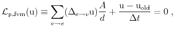where $\Delta t$ denotes the time step and $\mathrm{u}_{\mathrm{old}}$ stands for the solution function $\mathrm{u}$ in the prior time step. This scheme is known as the implicit Euler time discretization. The explicit time discretization, which avoids the solution of an equation system but becomes unstable if time steps are too large, is formulated analogously:

$$\mathcal{L}_\mathrm{p\_fvm}(\mathrm{u}) \equiv \sum_{v\rightarrow... ...) \frac{A}{d} + \frac{\mathrm{u} - \mathrm{u}_{\mathrm{old}}}{\Delta t} = 0 \;.$$

The GSSE diffusion application is available for two and three dimensions, as well as for structured grids and unstructured meshes, which are demonstrated in the following by two different examples.

8.3.2 Transformation into the GSSE 

By using the finite volume method and the specification mechanism enabled by the GSSE, the next code snippet shows a possible implementation. Here, the boundary evaluation is also shown where the conditional statements are based on abstract quantities, as illustrated in Section 8.1. First, the implicit time discretization and the corresponding specification is given. The domaintype tag is also available by the GSSE .

The Dirichlet boundary condition is specified by the abstract boundary condition quantity u_bnd. An explicit time discretizaton is presented next, where the resuability of developed components can be easily observed. Almost the entire implementation can be reused, whereas the functional paradigm enables the exchange of only one quantity accessor.

8.3.3 Results

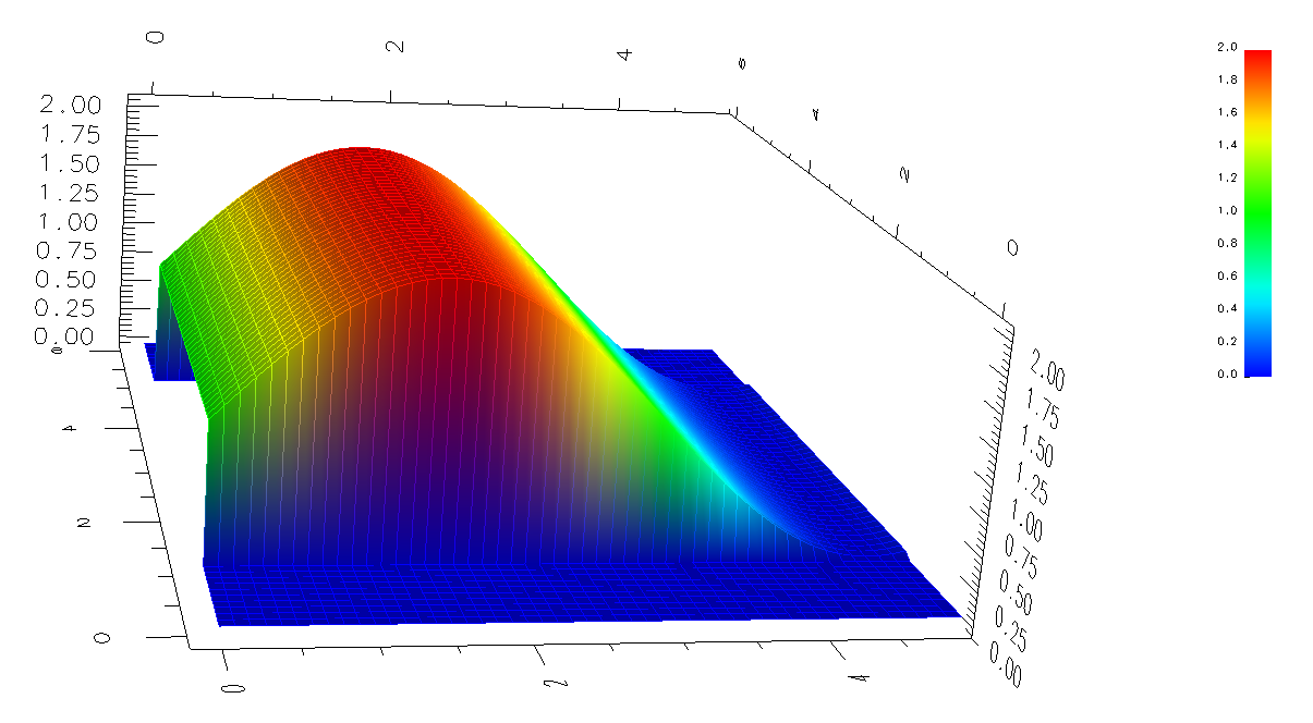
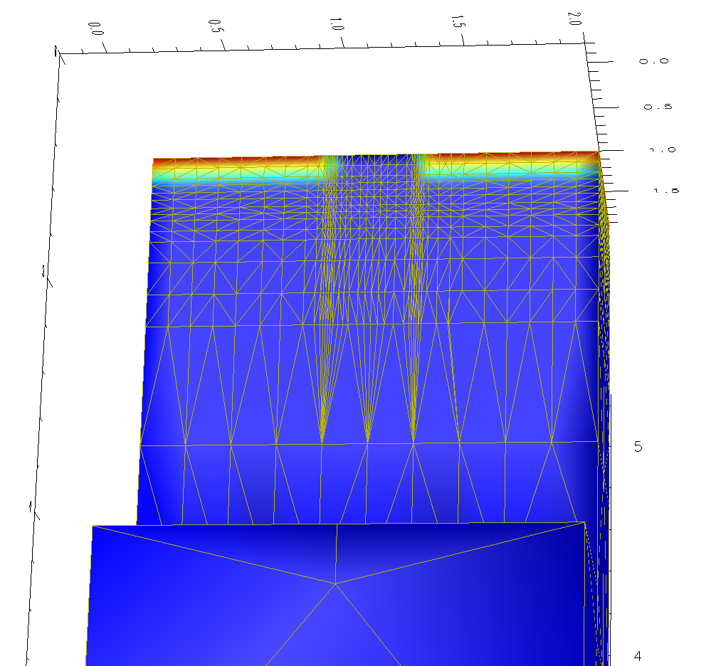
In two dimensions, a structured grid (see Figure 8.9) is used, and the influence of the boundary conditions is shown. The left side of the simulation domain ($x=0$ ) is used as a constant source of diffusion particles, thereby creating a steady flow into the area. All other boundaries are modeled by a Neumann boundary condition.

Figure 8.9: Two-dimensional structured grid with an initial doping profile (concentration in $\textnormal {cm}^{-1}$).

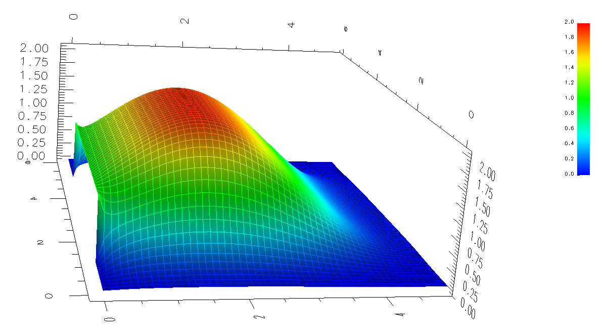
The simulation results for two subsequent time steps are given in Figure 8.10 and Figure 8.11.

Figure 8.10: Two-dimensional diffusion simulation for a structured grid after $200$ time steps.

Figure 8.11: Two-dimensional diffusion simulation for a structured grid after $2000$ time steps.

The three-dimensional unstructured mesh example, depicted in Figure 8.12, is based on an analytic ion-implantation module, which also generated the point cloud automatically [153]. The corresponding mesh generation, input preparation for the analytic ion implantation and dual mesh calculation, and simulation times are given in the following table (AMD X2, see Section 7.4 for more details):

Task	Number of points	Time [s]
mesh generation	$3 10^{3}$	$2.7$
input preparation		$18.1$
diffusion simulation		$18.2$

Figure 8.12: Three-dimensional device structure with an initial phosphorus doping profile (concentration in $\textnormal {cm}^{-1}$ ).

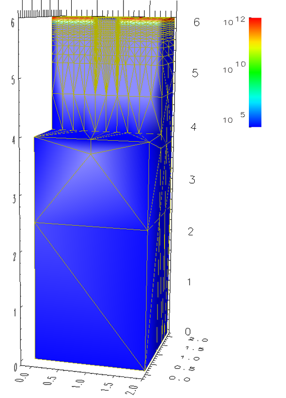Two subsequent diffusion steps are depicted in Figure 8.13, which are used as a rapid annealing step after ion implantation [69].

Figure 8.13: Three-dimensional diffusion simulation for a device structure with an initial doping profile. Two subsequent simulation steps are depicted.