4.1.3 Fourier Analysis of an Imaging System

In the preceding two sections diffraction phenomena in the optical far field and the imaging properties of a single thin converging lens were studied. The resulting formulae (4.11) and (4.19) establish linear relations between the optical field at different spatial coordinates. 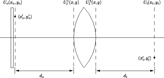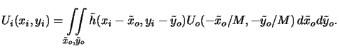In view of this linearity of the wave propagation phenomenon, a general linear superposition integral is postulated to describe imaging formation with a lens configuration similar to that shown in Figure 4.4. The image amplitude U_i(x_i, y_i) is related to the object amplitude U_o(x_o, y_o) by

 

$$U_i(x_i,y_i)=\iint\limits_{x_o,y_o} h(x_i,y_i;x_o,y_o) U_o(x_o,y_o)\, dx_ody_o,$$ (4.21)

whereby (x_i, y_i) and (x_o, y_o) are the image and object coordinates, respectively. Theoretically, the kernel h(x_i, y_i;x_o, y_o) equals the image amplitude U_i(x_i, y_i), if the object is an ideal unit-amplitude point source located at (x_o^$\prime$, y_o^$\prime$), i.e.,

$${U_i(x_i,y_i) = h(x_i,y_i;x_o^\prime,y_o^\prime)}{}\qquad{\text{for}}\qquad{} U_o(x_o,y_o) = \delta(x_o-x_o^\prime) \delta(y_o-y_o^\prime).$$ (4.22)

  

Figure 4.4: Image formation with a lens. The image amplitude U_i(x_i, y_i) is related to the object amplitude U_o(x_o, y_o) by a linear superposition integral.

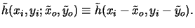
How can we determine the kernel h(x_i, y_i;x_o, y_o) in practice?^g First, we recall that a spherical wave diverging from the point source travels towards the lens. The amplitude incident on the lens is given by

$$U_l^1(x_l,y_l) = \frac{e^{j\frac{k_0}{2d_o}\left((x_l-x_o)^2+(y_l-y_o)^2\right)}}{j\lambda d_o},$$ (4.23)

whereby we have readily employed the paraxial approximation. After passage through the lens, the field distribution writes with (4.19) and (4.21) as

$$U_l^2(x_l,y_l) = e^{-j\frac{k_0}{2f}\left(x_l^2+y_l^2\right)} \, \mathcal{P}(x_l,y_l) \, U_l^1(x_l,y_l).$$ (4.24)

Finally, the image amplitude is given by the Fresnel approximation of (4.14),

$$U_i(x_i,y_i) = \frac{j}{\lambda d_i} \iint\limits_{x_l,y_l} U_l^2(x_l,y_l) e^{j\frac{k_0}{2d_i}\left((x_i-x_l)^2+(y_i-y_l)^2\right)}\,dx_ldy_l.$$ (4.25)

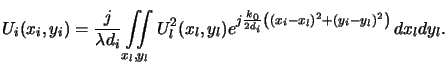
The impulse response looked for follows now from the above three equations to

 

$$h(x_i,y_i;x_o,y_o) \cong \frac{1}{\lambda^2 d_o d_i} \iint\limits... ...ight)x_l + \left(\frac{y_o}{d_o}+\frac{y_i}{d_i}\right)y_l \right]} \,dx_ldy_l,$$ (4.26)

whereby we have neglected the two quadratic phase factors ${\frac{k_0}{2d_i}}$(x_i² + y_i²) and ${\frac{k_0}{2d_o}}$(x_o² + y_o²). The first factor ${\frac{k_0}{2d_i}}$(x_i² + y_i²) can be eliminated by noting that we are primarily interested in the intensity distribution of the image, i.e., in the square module of the image amplitude. The second phase factor ${\frac{k_0}{2d_o}}$(x_o² + y_o²) cannot simply be dropped as it depends on the integration variables (x_o, y_o) of (4.24). However, assuming that the image amplitude at (x_i, y_i) consists only of object contributions from a tiny region located around (x_o, y_o) = - M(x_i, y_i), we approximately get exp(${\frac{k_0}{2d_o}}$(x_o² + y_o²)) $\approx$ exp(${\frac{k_0}{2d_oM^2}}$(x_i² + y_i²)). The quantity M is the magnification of the system and will be defined soon (cf. (4.31)). Because the dependence on the object space coordinates has been removed, the second phase factor can be dropped following the same arguments as for the first one.

As a final simplification, we restrict our attention to a particular plane behind the lens, namely that for which the image plane distance d_i satisfies

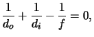$$\frac{1}{d_o}+\frac{1}{d_i}-\frac{1}{f} =0,$$ (4.27)

and 1/f > 1/d₀ so that 1/d_i = 1/f - 1/d₀ > 0 holds. This relation is well-known in geometrical optics and is usually called the lens law. To achieve a compact and physically predicative form for the kernel (4.29) we now introduce the magnification of the projection system as

 

$$M \overset{\mathrm{def}}{=}\frac{d_i}{d_o}.$$ (4.28)

Using the magnification thus defined to scale the object coordinates and introducing spatial frequencies for the lens coordinates,

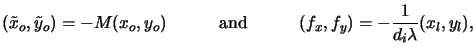$$(\tilde{x}_o,\tilde{y}_o) = -M(x_o,y_o){}\quad\qquad{\text{and}}\qquad\quad{}(f_x,f_y) = -\frac{1}{d_i\lambda}(x_l,y_l),$$ (4.29)

a scaled version $\tilde{h}$(x_i, y_i;$\tilde{x}_{o}^{}$,$\tilde{y}_{o}^{}$) of the kernel (4.29)^h

 

$$\tilde{h}(x_i,y_i;\tilde{x}_o,\tilde{y}_o) \cong M\iint\limits_{f... ..._y) e^{j2\pi\left[(x_i-\tilde{x}_o)f_x+(y_i-\tilde{y}_o)f_y\right]} \,df_xdf_y.$$ (4.30)

This relation is of fundamental importance for the Fourier analysis of an imaging system as it not only determines the kernel of the superposition integral (4.24), but also shows the shift-invariance of it, i.e.,

$$\tilde{h}(x_i,y_i;\tilde{x}_o,\tilde{y}_o) \equiv \tilde{h}(x_i-\tilde{x}_o,y_i-\tilde{y}_o).$$ (4.31)

This means that the relation between object and image field is a convolution integral,

 

$$U_i(x_i,y_i) = \iint\limits_{\tilde{x}_o,\tilde{y}_o} \tilde{h}(x... ...i-\tilde{y}_o) U_o(-\tilde{x}_o/M,-\tilde{y}_o/M) \, d\tilde{x}_o d\tilde{y}_o.$$ (4.32)

As can be seen from (4.33) the kernel or the impulse response $\tilde{h}$(x, y) is the inverse Fourier transformⁱ of a scaled version of the pupil function $\mathcal {P}$(x, y), i.e.,

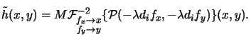$$\tilde{h}(x,y) = M\mathcal{F}^{-2}\begin{Sb}f_x\rightarrow x\\ f_y\rightarrow y \end{Sb} \{\mathcal{P}(-\lambda d_if_x,-\lambda d_if_y)\}(x,y).$$ (4.33)

With the convolution theorem^j of the Fourier transform we can transform (4.35) into the frequency domain and obtain the following simple relation between object and image spectrum:

 

$$\mathcal{F}^2\begin{Sb}x\rightarrow f_x\\ y\rightarrow f_y \end{S... ...gin{Sb}x\rightarrow f_x\\ y\rightarrow f_y \end{Sb}\{U_o(-x/M,-y/M)\}(f_x,f_y).$$ (4.34)

This equation is in accordance with geometrical optics, since as $\lambda$ approaches zero the range over which $\mathcal {P}$(- $\lambda$d_if_x, - $\lambda$d_if_y) equals unity will grow without bounds allowing it to be replaced by unity. Hence, in the limiting case $\lambda$ $\rightarrow$ 0 the object and image are related by U_i(x, y) = MU_o(- x/M, - y/M), i.e., the image is an exact replica of the object, magnified and inverted in the image plane.

Footnotes

... practice?^g

In the subsequent derivation (x_o, y_o) refers to the point source location in the object space instead of (x^$\prime$_o, y^$\prime$_o). The difference between the fixed location (x^$\prime$_o, y^$\prime$_o) and the coordinates (x_o, y_o) is clear throughout the discussion anyway.

...)^h

The scaled kernel is defined by $\tilde{h}$(x_i, y_i;$\tilde{x}_{o}^{}$,$\tilde{y}_{o}^{}$) = h(x_i, y_i; - $\tilde{x}_{o}^{}$/M, - $\tilde{y}_{o}^{}$/M).

... ⁱ

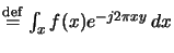The Fourier transform F(y) of a function f (x) is defined as F(y) = $\mathcal {F}$_{x $\rightarrow$ y}{f (x)}(y)$\overset{\mathrm{def}}{=} \int_xf(x)e^{-j2\pi xy}\,dx$ and its inverse is given by f (x) = $\mathcal {F}$^-1_{y $\rightarrow$ x}{F(y)}(x)$\overset{\mathrm{def}}{=} \int_yF(y)e^{j2\pi xy}\,dx$.

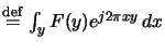... ^j

The convolution theorem states that the Fourier transform of a convolution integral (h*f )(x) = $\int_{x^\prime}^{}$h(x - x^$\prime$)f (x^$\prime$) dx^$\prime$ of two functions h(x) and f (x) equals the product of the two Fourier transforms H(y) and F(y), i.e., $\mathcal {F}$_{x $\rightarrow$ y}{(h*f )(x)}(y) = H(y) F(y).