From a theoretical point of view probability distributions are better described in terms of cumulants than in terms of moments, see [Rot01]. This motivated us to study the notion of cumulants and apply it to the closure problem. Using a cumulant expansion method for device simulation was also suggested in [WSYM98]. In [SH00], the cumulant method was used for the solution of the Boltzmann equation in the context of gas dynamics.
In probability theory and statistics, the cumulants
![]() of a probability distribution
of a probability distribution ![]() are given by
are given by
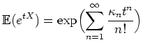 |
(3.1) |
where ![]() is any random variable whose probability
distribution is the one whose cumulants are taken
and
is any random variable whose probability
distribution is the one whose cumulants are taken
and ![]() is a real parameter.
is a real parameter.
In other words,
![]() is the
is the ![]() -th
coefficient in the power series of the moment generating
function. The logarithm of the moment-generating function
is therefore called the cumulant-generating function.
-th
coefficient in the power series of the moment generating
function. The logarithm of the moment-generating function
is therefore called the cumulant-generating function.
Equivalently (via the complex domain)
cumulants can be defined by using the
characteristic function (Fourier transform of ![]() )
in place of the moment generating
function [Mat99].
)
in place of the moment generating
function [Mat99].
The first cumulant is equal to the logarithm of the total mass of the distribution function (hence zero for proper probability distribution functions). The second cumulant is the variance. Cumulants of order greater than 2 are measures of non-normality. The third and fourth cumulant are related to the skewness and the kurtosis, respectively. For a distribution function with unit variance the kurtosis is equal to the fourth cumulant. Calculations simplify if central moments are used.
In the cumulant expansion method closure of the highest order equation can be achieved by setting all higher cumulants to zero. This translates to a condition on the moments and defines a generalized Gaussian closure.
Application of this closure to our system of moment equations encounters technical difficulties. The reason is that the expression for the sixth moment from a general three-dimensional distribution function contains lower order moments which are not fixed by the reduced set of moments given in 2.22.
These difficulties can be overcome in two different ways. In the first way we assume that our distribution is of the linear-isotropic type Equation 2.17. With this constraint all lower-order moments are fixed and we can calculate the cumulant closure by using Ansatz 2.17 for the distribution function.
In the second method we use another class of distribution functions to fix all lower-order moments. We observed that the logarithm of the Fourier transform is a polynomial, when the cumulant closure is applied. By chance this family of distribution is formally the same as the ansatz derived from a maximum entropy closure. Hence in the second way we assume that the logarithm of the Fourier transform is a polynom whose terms are given by the known moments. Note that we have to add all moments from the integrability conditions 2.40 into the ansatz.
This gives the ansatz
| (3.2) |
where ![]() denotes the Fourier transform of the
(normalized) distribution function
denotes the Fourier transform of the
(normalized) distribution function ![]() .
.
Closure of the equations is implicitly achieved as by this ansatz
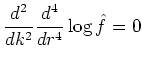 |
(3.3) |
 |
We note that using
an ansatz from the maximum entropy family
in Fourier space corresponding
to the isotropy condition does not work as not all higher
order derivatives exist at the origin due to the
occurrence of a square root ![]() in the distribution.
(The same holds true for the maximum entropy
class from the linear-isotropy condition.)
in the distribution.
(The same holds true for the maximum entropy
class from the linear-isotropy condition.)
The actual calculation consists of the manipulation
of some polynomial series expansion. This is in
principle straight forward, but gets involved in practice,
as terms up to order 6 in (![]() ) have to be considered.
Hence the calculations were implemented in
Mathematica.
) have to be considered.
Hence the calculations were implemented in
Mathematica.
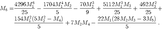
For the linear-isotropic ansatz we get the following closure
for ![]() :
:
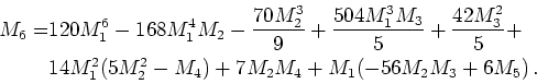 |
(3.4) |
From the ansatz stemming from the integrability conditions we get
 |
(3.5) |
Note that in these formulas we assume a normalized distribution. Assuming that all odd moments vanish in a diffusion approximation both formulas give the same closure:
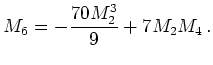 |
(3.6) |
Hence the cumulant closure is robust in a theoretical sense.
It can be checked that the diffusion cumulant closure
gives the correct value for ![]() in equilibrium.
in equilibrium.
The cumulant closure is a type of Gaussian closure
which is distinguished from a theoretical viewpoint.
It is given by a combination of closures
from Section 3.4
for values of ![]() and
and ![]() .
.
Within a cumulant expansion method the equilibrium type boundary conditions for the even moments are replaced by imposing zero Dirichlet boundary conditions for the even cumulants.
Furthermore the mobility and relaxation time models describing scattering can be replaced by descriptions in terms of cumulants [SH00].
![]()
![]()
![]()
![]() Previous: 3. Highest Order Moment
Up: 3. Highest Order Moment
Next: 3.2 Maximum Entropy Closure
Previous: 3. Highest Order Moment
Up: 3. Highest Order Moment
Next: 3.2 Maximum Entropy Closure