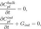
Although Blech had shown that electromigration transport was closely related to mechanical stress development, the first model that connected the rate of stress generation to electromigration was proposed by Kirchheim [53]. He added the gradient of mechanical stress as a driving force in the total vacancy flux equation, so that
The last term is a generation/annihilation function similar to that proposed by Rosenberg and Ohring [72], as shown in Section 2.3. However, Kirchheim used the more general expression for the equilibrium vacancy concentration in a grain boundary [84]
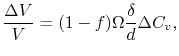
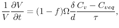
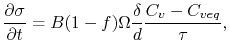
The volumetric strain in a grain produced by the generation of vacancies is [53]
This equation shows that the stress build-up is related to the deviation of the vacancy concentration from its equilibrium value and that
![]() can have a significant impact on the stress development. It is important to note that this model allows different mechanisms of vacancy annihilation or generation to be described, such as annihilation/production in the grain boundary itself, in adjacent grain boundaries or at dislocations within the grain bulk. These lead to smaller, median, and larger values of the characteristic vacancy relaxation time
can have a significant impact on the stress development. It is important to note that this model allows different mechanisms of vacancy annihilation or generation to be described, such as annihilation/production in the grain boundary itself, in adjacent grain boundaries or at dislocations within the grain bulk. These lead to smaller, median, and larger values of the characteristic vacancy relaxation time
![]() , respectively.
, respectively.
Equations (2.30) and (2.34) compose a non-linear system of differential equations, which has to be solved numerically. Nevertheless, Kirchheim derived analytical solutions for some limiting cases and identified three main phases for vacancy and stress evolution [53]. The first phase corresponds to a short period of time, where the initial stress is very low. Therefore, the equilibrium vacancy concentration remains unaffected and the vacancy concentration develops until a quasi steady-state condition is reached. The quasi steady-state phase is quite long, and the vacancy concentration does not change very much, while the stress grows linearly with time. It lasts until the stress becomes large enough to affect the equilibrium vacancy concentration. Then, a non-linear increase of stress with time is observed and the vacancy concentration approximately follows the development of the equilibrium vacancy concentration, which means that vacancies and stresses are in equilibrium and the true steady-state condition has been reached.
Moreover, Kirchheim [53] showed that, if the electromigration lifetime is determined by the time to reach a certain critical stress, the current density exponent of Black's equation varies from ![]() at low stresses (the time to failure is determined by the quasi steady-state period) to
at low stresses (the time to failure is determined by the quasi steady-state period) to ![]() for higher critical stresses (the time to reach the true steady-state condition determines the lifetime).
for higher critical stresses (the time to reach the true steady-state condition determines the lifetime).
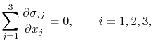
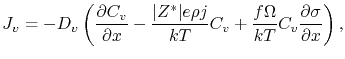
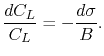
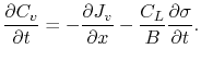
A somewhat simplified model for the stress development in a line subject to electromigration was derived by Korhonen et al. [54]. They consider that the generation/recombination of vacancies by dislocation climb mechanisms either in grain boundaries or at lattice dislocations changes the concentration of lattice sites, ![]() , producing stress according to Hooke's law
, producing stress according to Hooke's law
Korhonen et al. observed that
![]() at typical electromigration test conditions. This means that most of the transported vacancies initiate climbing dislocation processes which produce mechanical stress, while just a very small number of vacancies is needed to maintain the local equilibrium concentration [54]. Thus, the above approximation leads to
at typical electromigration test conditions. This means that most of the transported vacancies initiate climbing dislocation processes which produce mechanical stress, while just a very small number of vacancies is needed to maintain the local equilibrium concentration [54]. Thus, the above approximation leads to
For a line of length ![]() with blocking boundary conditions
with blocking boundary conditions
Following the same approach as Korhonen et al., Clement et al. [55,85] derived an equivalent equation in terms of vacancies,
Assuming that the electromigration failure is determined by the time to reach a given stress magnitude, the above models predict a mean time to failure of the form
Figure 2.1 shows the stress development with time at ![]() according to Korhonen's solution, (2.42).
Note that the time scale of stress build-up is in the order of several hours, rather than a few minutes as predicted by the models of Section 2.3.
This shows the importance of taking into account the mechanical stress in the model, including the stress dependence in the sink/source term of the continuity equation.
The stress distribution along the line for several times is presented in Figure 2.2. At steady-state the stress varies linearly, as predicted by Blech [75,76,77]. One can see that high stress can develop in the interconnect line, which is a critical requirement for void nucleation [88,89].
according to Korhonen's solution, (2.42).
Note that the time scale of stress build-up is in the order of several hours, rather than a few minutes as predicted by the models of Section 2.3.
This shows the importance of taking into account the mechanical stress in the model, including the stress dependence in the sink/source term of the continuity equation.
The stress distribution along the line for several times is presented in Figure 2.2. At steady-state the stress varies linearly, as predicted by Blech [75,76,77]. One can see that high stress can develop in the interconnect line, which is a critical requirement for void nucleation [88,89].
These models were very successful in explaining the origin of mechanical stress and calculating the hydrostatic stress which develops in a metal line due to electromigration. However, they are based on several simplifying assumptions and are applicable to simple interconnect lines only.
For example, the mechanical properties of the line and the effect of the constraints imposed by the surrounding materials are all taken into account by the modulus
![]() in the equations above.
Therefore, a more general description of the problem is required, in order to better understand the mechanical stress distribution and its effects on the interconnect structures.
in the equations above.
Therefore, a more general description of the problem is required, in order to better understand the mechanical stress distribution and its effects on the interconnect structures.
The connection between material transport with mechanical stress in a general framework was first proposed by Povirk [90] and Rzepka et al. [91]. In these works mass accumulation or depletion in the metal line leads to an inelastic strain rate of the form
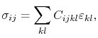
Sarychev et al. [92] extended this formulation considering that the total inelastic strain rate has a contribution from vacancy accumulation/depletion and a contribution from vacancy generation/annihilation, yielding
The key characteristic of Sarychev's approach is that it forms a three-dimensional self-consistent model which connects material balance with line deformation. In this way, the impact of the complete interconnect geometry and imposed boundary conditions on the stress evolution can be described. Furthermore, all components of the stress tensor can be determined. Sarychev's model was the basis of several works on simulation of stress evolution due to electromigration [93,94,95,96] in two-dimensional lines.
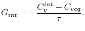
A different approach was proposed by Sukharev et al. [97,98,99,100], who introduced the concept of plated atoms to describe the atom exchange between bulk and interfaces. He suggested that the event of vacancy generation or annihilation is simultaneously accompanied by atom plating or removal from the grain boundary region, respectively. Therefore, the rate of atom plating/removal is given by the same source function as for vacancies,
Using this concept, the electromigration induced strain is written as [97]
![$\displaystyle \ensuremath{\ensuremath{\frac{\partial \CV}{\partial t}}} = -\ens...
... \symHydStress}{\partial x}}}\right) \right] - \frac{\CV-\Ceq}{\symVacRelTime}.$](img218.png)
![$\displaystyle \Ceq = \Co\exp\left[\frac{(1-\symVacRelFactor)\symAtomVol\symHydStress}{\kB\T}\right],$](img219.png)

![$\displaystyle \left(\frac{\CV\symBulkMod\symAtomVol}{\CL\kB\T} + 1\right) \frac...
...dStress}{\partial x}}} - \vert\Z\vert\ee\symElecRes\symCurrDens\right) \right],$](img232.png)
![$\displaystyle \ensuremath{\ensuremath{\frac{\partial \symHydStress}{\partial t}...
...}} - \frac{\vert\Z\vert\ee\symElecRes\symCurrDens}{\symAtomVol}\right) \right],$](img235.png)
![$\displaystyle \symHydStress(x,t) = \frac{\vert\Z\vert\ee\symElecRes\symCurrDens...
...-m_n^2\frac{\kappa}{\symL^2}t\right)\cos\left(m_n\frac{x}{\symL}\right)\right],$](img238.png)

![$\displaystyle \symHydStress(x,t) = \frac{\kB\T}{\symAtomVol}\ln\left[\frac{\CV(x,t)}{\Co}\right],$](img243.png)
![\includegraphics[width=0.80\linewidth]{chapter_physics_EM/Figures/K_str_t.eps}](img249.png)
![\includegraphics[width=0.80\linewidth]{chapter_physics_EM/Figures/K_str_x.eps}](img250.png)
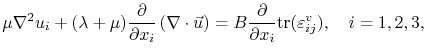
![$\displaystyle \ensuremath{\ensuremath{\frac{\partial \symStrain^{v}_{ij}}{\part...
...\ensuremath{\nabla\cdot{\vec\JV}} + (1-\symVacRelFactor)\G\right]\symKronecker.$](img253.png)