4.2.1 Discretization of Laplace's Equation

The electric potential is calculated from equation (3.71). Multiplying it by a test function ${\symShapeFun}_{p}={\symShapeFun}_{p}(\vec r)$, and integrating over the domain $\symDomain$ one obtains

$$\ensuremath{\int_{\symDomain}{\left[\ensuremath{\nabla\cdot{(\sym... ...symElecPot}})}}\right]{\symShapeFun}_{p}}\ d{\symDomain}} = 0,\qquad p=1,...,N.$$ (4.25)

Using Green's formula [152]

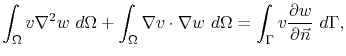$$\ensuremath{\int_{\symDomain}{v\ensuremath{\nabla^2 w}}\ d{\symDo... ...mBoundary}{v\ensuremath{\frac{\partial w}{\partial \vec n}}}\ d{\symBoundary}},$$ (4.26)

where $\partial{w}/\partial{\vec n}$ represents the normal derivative in the outward normal direction to the boundary $\symBoundary$, and assuming a Neumann boundary condition, i.e. vanishing normal derivatives, on $\symBoundary$, equation (4.25) can be written as

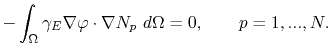$$-\ensuremath{\int_{\symDomain}{\symElecCond\ensuremath{\nabla{\sy... ...}\ensuremath{\nabla{{\symShapeFun}_{p}}}}\ d{\symDomain}} = 0,\qquad p=1,...,N.$$ (4.27)

Since the electrical conductivity $\symElecCond$ depends on the temperature according to (3.73) and varies along the simulation domain, it is part of the integrand in (4.27). However, in a single element the conductivity is assumed to be constant, being determined by the average of the temperature on the element nodes, i.e. $\symElecCond = \symElecCond(\bar\T)$ with

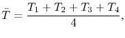$$\bar\T = \frac{{\T}_{1} + {\T}_{2} + {\T}_{3} + {\T}_{4}}{4},$$ (4.28)

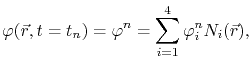
for a tetrahedral element. Applying the discretization for the electric potential as in (4.6),

$$\symElecPot(\vec r, t=t_n) = \symElecPot^n = \ensuremath{\sum_{i=1}^{4}{\symElecPot_i^n}}{\symShapeFun}_{i}(\vec r),$$ (4.29)

where $\symElecPot_i^n$ is the electric potential of the node $i$ at a time $t_n$, equation (4.27) for a single element becomes

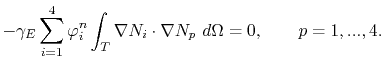$$-\symElecCond\ensuremath{\sum_{i=1}^{4}{\symElecPot_i^n}} \ensure... ...}\ensuremath{\nabla{{\symShapeFun}_{p}}}}\ d{\symDomain}} = 0,\qquad p=1,...,4.$$ (4.30)

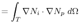
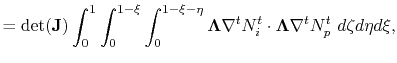
Using the shorthand notation

$$K_{ip} = \ensuremath{\int_{T}{\ensuremath{\nabla{{\symShapeFun}_{i}}}\ensuremath{\cdot}\ensuremath{\nabla{{\symShapeFun}_{p}}}}\ d{\symDomain}}$$

$$= \det(\mathbf{J})\int_{0}^{1}\int_{0}^{1-\xi}\int_{0}^{1-\xi-\et... ...\ensuremath{\cdot}\mathbf{\Lambda}\nabla^t \symShapeFun_p^t\ d\zeta d\eta d\xi,$$ (4.31)

where the last term is the calculation in the transformed coordinate system, (4.30) is rewritten as

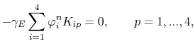$$-\symElecCond\ensuremath{\sum_{i=1}^{4}{\symElecPot_i^n}}K_{ip} = 0, \qquad p=1,...,4,$$ (4.32)

which corresponds to a discrete system of 4 equations with 4 unknowns, i.e. the electric potential at each node of the tetrahedral element.