Next: 4.2.3 Discretization of the
Up: 4.2 Discretization of the
Previous: 4.2.1 Discretization of Laplace's
4.2.2 Discretization of the Thermal Equation
For convenience, the thermal equation (3.72) is rewritten here as
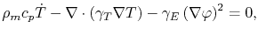 |
(4.33) |
where the notation
 is used.
Following the same procedure as for Laplace's equation, one multiplies (4.33) by
is used.
Following the same procedure as for Laplace's equation, one multiplies (4.33) by
 and integrates over the domain
 , which together with Green's formula (4.26) and a Neumann boundary condition yields the weak formulation
 |
(4.34) |
The thermal equation (4.33) corresponds to a parabolic problem. Besides the spatial discretization, a discretization in time has also to be performed. A simple choice is the backward Euler method
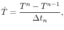 |
(4.35) |
where
 is the time step. Applying now the spatial discretization for the temperature variable
 |
(4.36) |
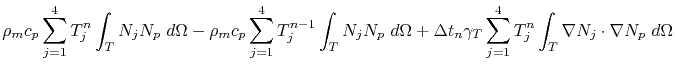
and the electric potential discretization (4.29), equation (4.34) is written for a single element as
| |
 |
|
| |
 |
(4.37) |
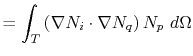
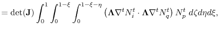
Using the integral notations (4.31),
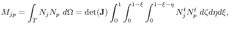 |
(4.38) |
and
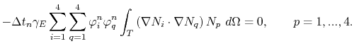
(4.37) can be expressed as
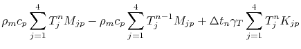 |
|
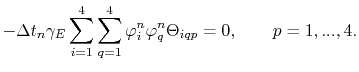 |
(4.40) |
This is the discrete system of equations, which has to be solved each time step in order to obtain the temperature at each node of the element.
Next: 4.2.3 Discretization of the
Up: 4.2 Discretization of the
Previous: 4.2.1 Discretization of Laplace's
R. L. de Orio: Electromigration Modeling and Simulation