Dissertation — Bottom-Up Correction for Re-Distancing

Chapter 7 Bottom-Up Correction for Re-Distancing

The previous chapter presented an algorithm used in the Re-Distancing step in a top-down manner (processing the levels of a hierarchical grid from coarsest to finest). In contrast, this chapter proposes a bottom-up correction algorithm to increase the accuracy of the signed-distance field on coarser levels of the hierarchical grid. This is important to couple the levels of the hierarchical grid together, because Re-Gridding may remove higher levels from the hierarchical grid. An additional goal is to keep the computational overhead low with respect to the always necessary top-down re-distancing algorithm. The developed algorithm does not only increase the accuracy in regions covered by blocks on a higher level, as is possible through straightforward interpolation, but also in regions not covered by blocks on higher levels.

First, the idea and the algorithmic implementation of the proposed bottom-up correction algorithm, which is the core contribution of this chapter [100], is discussed (Section 7.1). Then the proposed bottom-up correction algorithm is evaluated, by two criteria (Section 7.2):

• Accuracy: Computing the errors (difference to an exact solution) of the signed-distance field.
• Performance: Measuring the run-time compared to Re-Distancing without the correction algorithm.

The evaluation examples consider interfaces representing typical challenges in process TCAD simulations, i.e., corners and trenches. The examples are prepared and chosen so as to allow for the exact computation of a signed-distance field as explicit interface representations (e.g., triangles) are available.

7.1 Algorithmic Implementation

The core idea of the developed bottom-up correction algorithm is to process the levels of a hierarchical grid in reversed order. The reversed order allows to incorporate the solution from spatially fine resolved regions into coarse resolved regions.

The algorithm (cf. Algorithm 10) operates in a bottom-up manner, starting from the second highest level: The highest level may not be corrected, because there is no higher level from which to derive a correction. First, the signed-distance field is interpolated based on the solution on the higher level of the hierarchical grid and then the FMM is used to improve the accuracy of the signed-distance field. The usage of the FMM allows to improve the accuracy in regions which are not covered by blocks on higher levels.

1 procedure Correction():

2 $l \leftarrow$ highest level -1

3 while $l \geq 0$ do

/* Initialization Phase */

4 foreach Block on Level $l$ do // Parallel region

5 foreach ChildBlock on Level $l + 1$ do // Nested parallel region

6 InterpolatedLists $\leftarrow$ interpolateGridPoints() // Create task

7 end foreach

8 mergeInterpolatedLists()

9 initializeFMMCorrection()

10 end foreach

11 Wait // Synchronization barrier

/* Marching Phase */

12 foreach Block on Level $l$ do // Unmodified marching

13 Marching() // Create task

14 end foreach

15 Wait // Synchronization barrier

16 $l \leftarrow l - 1$ // Move to next level

17 end while

18 end procedure

Algorithm 10: The bottom-up correction algorithm processes the hierarchical grid in a bottom-up manner. First, the signed-distance field on a level is interpolated based on the solution of the next higher level. Then the FMM is initialized keeping the flags from the previous (top-down) re-distancing. Finally, an unmodified marching (from the FMM) is used to correct the solution also in unrefined regions.

In a practical setting, the overhead of the bottom-up correction algorithm is reduced by reusing the flags (adapting the initialization of the FMM) used by the presented (top-down) algorithm in Section 5.3. On every level the developed algorithm is split into two phases (same phases as the FMM):

• Initialization: Interpolation of the signed-distance values based on the values on higher levels and collect the corresponding grid points in block-specific lists. Those lists are then used to initialize the Band data structure (Heap).
• Marching: Execute the core multi-block FMM. For efficiency purposes grid points keep their signed-distance value and flag from the previous top-down re-distancing algorithm.

Initialization

The initialization phase starts in Algorithm 10 Line: 4. All blocks on the current level (Level $l$ ) are processed in parallel. For each block on the current level a nested parallel region for all its child blocks is created. With the nested parallel region the interpolation is able to utilize the usually higher number of blocks on higher levels of a hierarchical grid (Level ( $l + 1$ )) for a better load-balancing and, therefore, a better parallelization.

The $Φ$ values of grid points covered by a block on the next higher level are interpolated using a linear interpolation along all spatial directions. Thus, bilinear interpolation in 2D simulations and trilinear interpolation in 3D simulations. In Figure 7.1 a schematic representation of the interpolation cases is shown: The interface is shown by the green curves on both levels (the higher spatial resolution on the higher level allows for a more accurate, i.e., sharper, representation of corners). The red dots mark grid points on the outside and blue ones on the inside. The grid points on the lower level are labeled with a letter from A to L. Some of the cells on the higher level are not marked with a colored point, because the signed-distance field has been computed only in a narrow-band¹. However, on a hierarchical grid the blocks on levels higher than zero, typically already form a narrow-band like structure. Thus, setting the narrow-band based on an explicit threshold value is rarely encountered on block based AMR, nevertheless still possible, therefore the case is also considered.

The grid points A, E, and I are not covered by a block on a higher level and, therefore, not interpolated. The grid points G, H, J, K, and L have a neighboring grid point with opposing sign. Thus, they are Close Points and must not be modified. The grid point B is also not interpolated as it is not fully covered by the computed values of the narrow-band on the higher level. The remaining grid points C, D, and F are interpolated.

In case of parallelization, there are no restrictions with respect to synchronizations (race conditions) because the nesting criteria of the hierarchical grid enforce that grid points are uniquely refined, i.e., each grid point on the lower level is interpolated by a dedicated set of grid points on the higher level. The interpolated points are first collected in a separate list: One list per block on the higher level. The lists are then merged through a reduction operation, so that for each block on the current level a single list is created containing all interpolated points on the block (Algorithm 10 Line: 8).

Afterwards the merged list of interpolated grid points is used to initialize the multi-block FMM [62]. The initialization is different compared to the multi-block FMM, because all grid points keep their current $Φ$ value and their current flag. Only the grid points from the merged list are set to Known and inserted into the Heap.

¹ For the level-set method it is sufficient to solve the level-set equation only in a narrow-band around the interface (on grid points where the absolute distance to the interface is less than a given threshold); this is done for efficiency purposes

Marching

Subsequently, the unmodified marching of the FMM is performed until all the heaps are empty (cf. Algorithm 10 Line: 12). The specialized initialization avoids the re-computation of all grid points, because a re-computation of all grid points would result in an approximately doubled run-time per level compared to the Re-Distancing step without correction algorithm. The main disadvantage of this approach is that grid points for which the distance to the interface has been under-estimated are not corrected. This is inherent to the FMM because grid points are only processed, if their newly computed distance is lower than their current one. However, this is only a minor issue because the FMM tends to over-estimates the distance [169].

After a global synchronization barrier (ensuring all heaps are empty), the algorithm eventually moves to the next level by decreasing the level counter $l$ by one Algorithm 10 Line: 16. The algorithm terminates when Level 0 is reached and corrected.

7.2 Benchmark Examples and Analyses

The effect of the bottom-up correction algorithm on the accuracy is first analyzed on 2D examples. Additionally, a 3D example is used to study the performance impact.

The accuracy is measured by computing the error (difference of the signed-distance field to an exact solution) in three discrete norms

$\begin{aligned} (7.1) & L_{1} -norm & : & \sum_{i \in I} | Φ_{i} - Φ |, \\ (7.2) & L_{2} -norm & : & \sqrt{\sum_{i \in I} {(Φ_{i} - Φ)}^{2}}, \\ (7.3) & L_{\infty} -norm & : & inf_{i \in I} | Φ_{i} - Φ | . \end{aligned}$ $Φ$ is the exact solution, while $Φ_{i}$ is the discrete approximation and the index set $I$ is given by the considered grid points, i.e., all nodes on a level of the hierarchical grid. The 2D examples consist of two corner examples (Corner and Sharp corner) providing basic insights on the bottom-up correction algorithm and the 2D Trench example (a typical geometry in process TCAD) highlights issues arising from thin trenches. The 3D example 3D Trench is a combination of the trench and corner geometries. Due to its higher computational load it is also used to evaluate the performance impact of the bottom-up correction algorithm.

The domain for all benchmark examples is chosen as $[- 1, 1]^{d}$ with $d \in {2, 3}$ with symmetric boundary conditions. For the 2D examples the domain is discretized using 40 grid points in all spatial directions on Level 0 and a refinement factor of four is used for both refinement level (Level 1 and Level 2). The 3D example has higher spatial discretization (50 grid points) on Level 0. The other grid settings are the same as in the 2D examples. The accuracy is compared to the exact solution computed using the explicit representations, i.e., triangles and lines for two and three dimensions, respectively. The exact solution is also used as the initial data of the Close Points utilized in the Re-Distancing step.

7.2.1 Corner

The Corner and Sharp corner examples have a corner located near the center of the domain. The corner as well as the sides of the angle are purposely not aligned to the computational grid to account for the generic case of a level-set simulation. The angle of the Corner example is 110° and for the Sharp corner example 50°. Figure 7.2 shows the level-set values together with several iso-lines extracted form Level 0 and the block placement (yellow rectangles) for both corner examples. On each level of the hierarchical grid only a single block is present, which is located around the corner near the center of the domain. In regions with low curvature only the black iso-line is visible, because all three solutions match and, therefore, their iso-lines overlap.

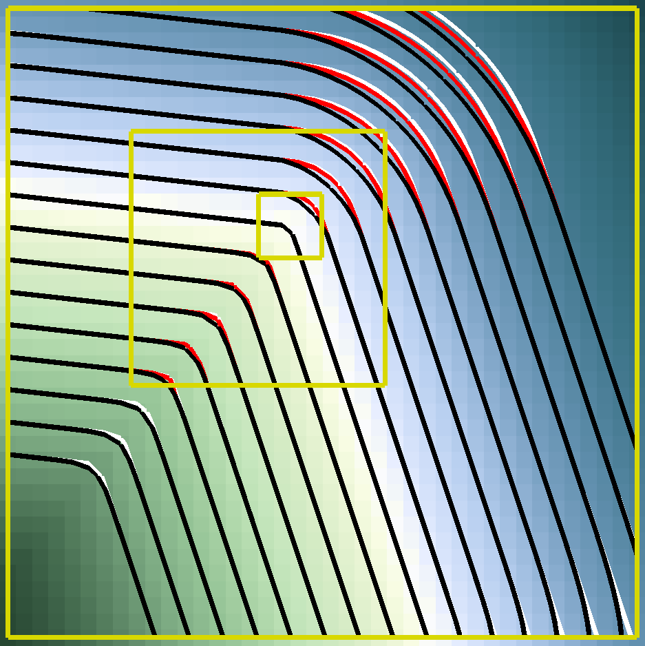
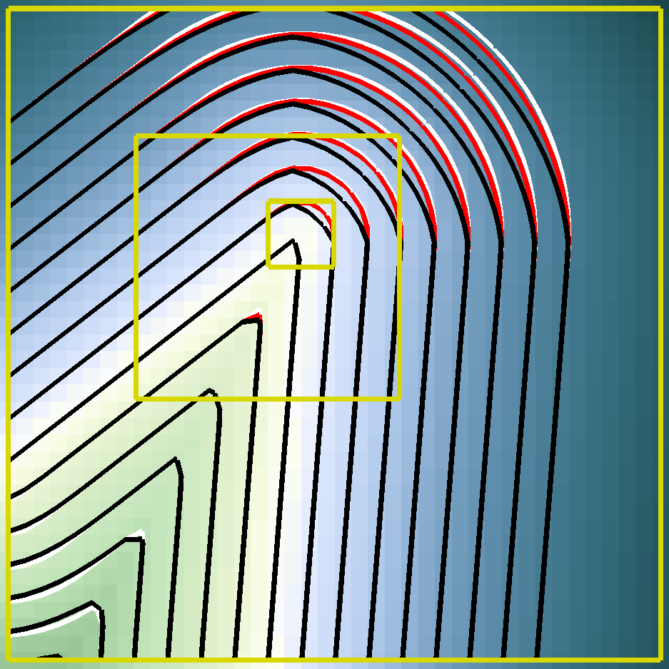
The symmetric boundary conditions which are applied to the lateral domain dimensions create additional corners at the domain boundary. Around these corners purposely no refinement is made (no block placed), therefore, the signed-distance field is not corrected around those corners: This allows for evaluating the effect precisely for a single corner. Generally speaking, the first-order approximation computed by the FMM over-estimates the distance to the interface for rarefaction fans (reflex angle side) and under-estimates the distance to the interface for shock waves (obtuse and acute angle side). The bottom-up correction algorithm increases the accuracy of the signed-distance field on rarefaction fans even outside the refined regions, due to the marching.

In Table 7.1 and Table 7.2 the error norms and the reduction by the proposed bottom-up correction algorithm are shown. For the Corner example the $L_{1}$ -norm and $L_{2}$ -norm errors are reduced by a factor of at least 2.1 on Level 0 and by a factor of 1.8 on Level 1. The Sharp Corner example shows an even higher reduction, 2.7 on Level 0 and 2.1 on Level 1, because sharper corners benefit more from the bottom-up correction algorithm. On Level 2 no correction is possible because it is the highest level.

Table 7.1: Error norms for the Corner example, with and without the bottom-up correction algorithm applied, and the corresponding factor by which the error norm is reduced. Adapted with permission from Springer Nature: Springer Cham, Quell et al., Studies in Computational Intelligence 902 (2021), pp. 438-451. [100], © 2021, under exclusive license to Springer Nature Switzerland AG.


Level	$L_{1}$ -norm	L1-reduc.	$L_{2}$ -norm	L2-reduc.	$L_{\infty}$ -norm	inf-reduc.


0	5.437e-3		3.260e-4		4.785e-2
0 corrected	2.491e-3	2.2	1.550e-4	2.1	3.079e-2	1.6
1	1.122e-3		5.101e-5		1.393e-2
1 corrected	6.035e-4	1.9	2.792e-5	1.8	8.541e-3	1.6
2	5.126e-4		1.819e-5		3.757e-3

Table 7.2: Error norms for the Sharp Corner example, with and without the bottom-up correction algorithm applied, and the corresponding factor by which the error norm is reduced. Adapted with permission from Springer Nature: Springer Cham, Quell et al., Studies in Computational Intelligence 902 (2021), pp. 438-451. [100], © 2021, under exclusive license to Springer Nature Switzerland AG.


Level	$L_{1}$ -norm	L1-reduc.	$L_{2}$ -norm	L2-reduc.	$L_{\infty}$ -norm	inf-reduc.


0	9.110e-3		4.823e-4		6.212e-2
0 corrected	3.388e-3	2.7	1.812e-4	2.7	2.707e-2	2.3
1	1.894e-3		7.264e-5		1.753e-2
1 corrected	8.957e-4	2.1	3.484e-5	2.1	9.546e-3	1.8
2	8.866e-4		2.569e-5		4.661e-3

7.2.2 Two-Dimensional Trench

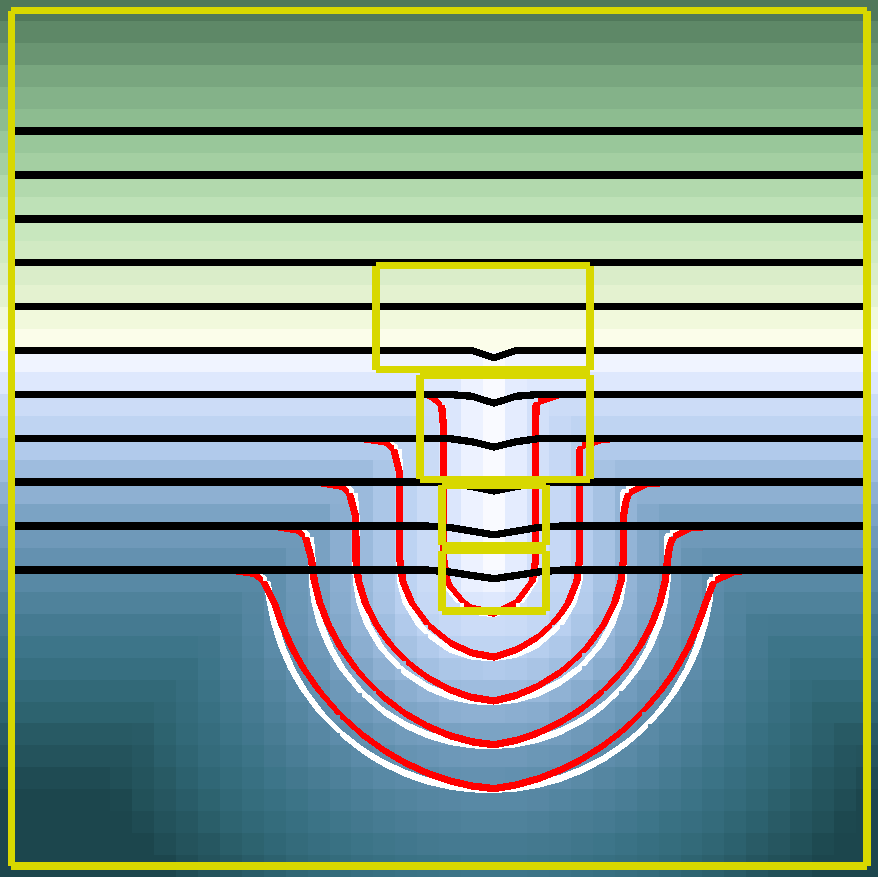
The 2D Trench is an axis-aligned thin trench on an otherwise flat surface. The interesting fact about this trench is the small width of only 0.001, because the Level 0 grid has only a spatial resolution of 0.05, thus is not able to resolve the trench, because no grid points with opposing sign exist along the trench. There are four blocks on Level 1 and six on Level 2, covering the trench completely and, therefore, enable the interface representation.

Such high aspect ratio trenches, are common in semiconductor manufacturing [191, 120] and thus by extension also in process TCAD simulations.

As shown in Figure 7.3 the Re-distancing step without the bottom-up correction algorithm shows only a small dent of the level-set on Level 0, while with the bottom-up correction algorithm the trench is well-resolved and present. This yields a significant reduction in the measured error norms (cf. Table 7.3): A reduction of 15.3 and 14.4, respectively for the $L_{1}$ -norm and $L_{2}$ -norm on Level 0. The impact on Level 1 is less (reduction of the error norms of 1.6) compared to the effect on Level 0, because the trench is able to be resolved natively on this level. The accuracy on this level is mainly increased at the rarefaction fans created by the two corners forming the bottom of the trench. The reduction of the error norm is lower compared to the Corner examples, because the rarefaction fans cover relatively (to the total number of grid points on a level) a smaller number of grid points.

Table 7.3: Error norms for the 2D Trench example, with and without the bottom-up correction algorithm applied, and the corresponding factor by which the error norm is reduced. Adapted with permission from Springer Nature: Springer Cham, Quell et al., Studies in Computational Intelligence 902 (2021), pp. 438-451. [100], © 2021, under exclusive license to Springer Nature Switzerland AG.


Level	$L_{1}$ -norm	L1-reduc.	$L_{2}$ -norm	L2-reduc.	$L_{\infty}$ -norm	inf-reduc.


0	9.101e-2		4.539e-3		4.839e-1
0 corrected	5.941e-3	15.3	3.148e-4	14.4	4.005e-2	12.1
1	6.732e-4		5.222e-5		1.262e-2
1 corrected	4.129e-4	1.6	3.339e-5	1.6	8.398e-3	1.5
2	6.709e-5		4.236e-6		3.400e-3

7.2.3 Three-Dimensional Trench

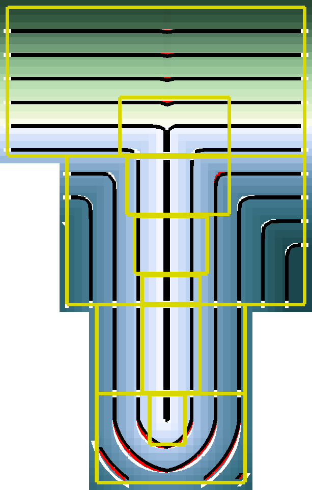
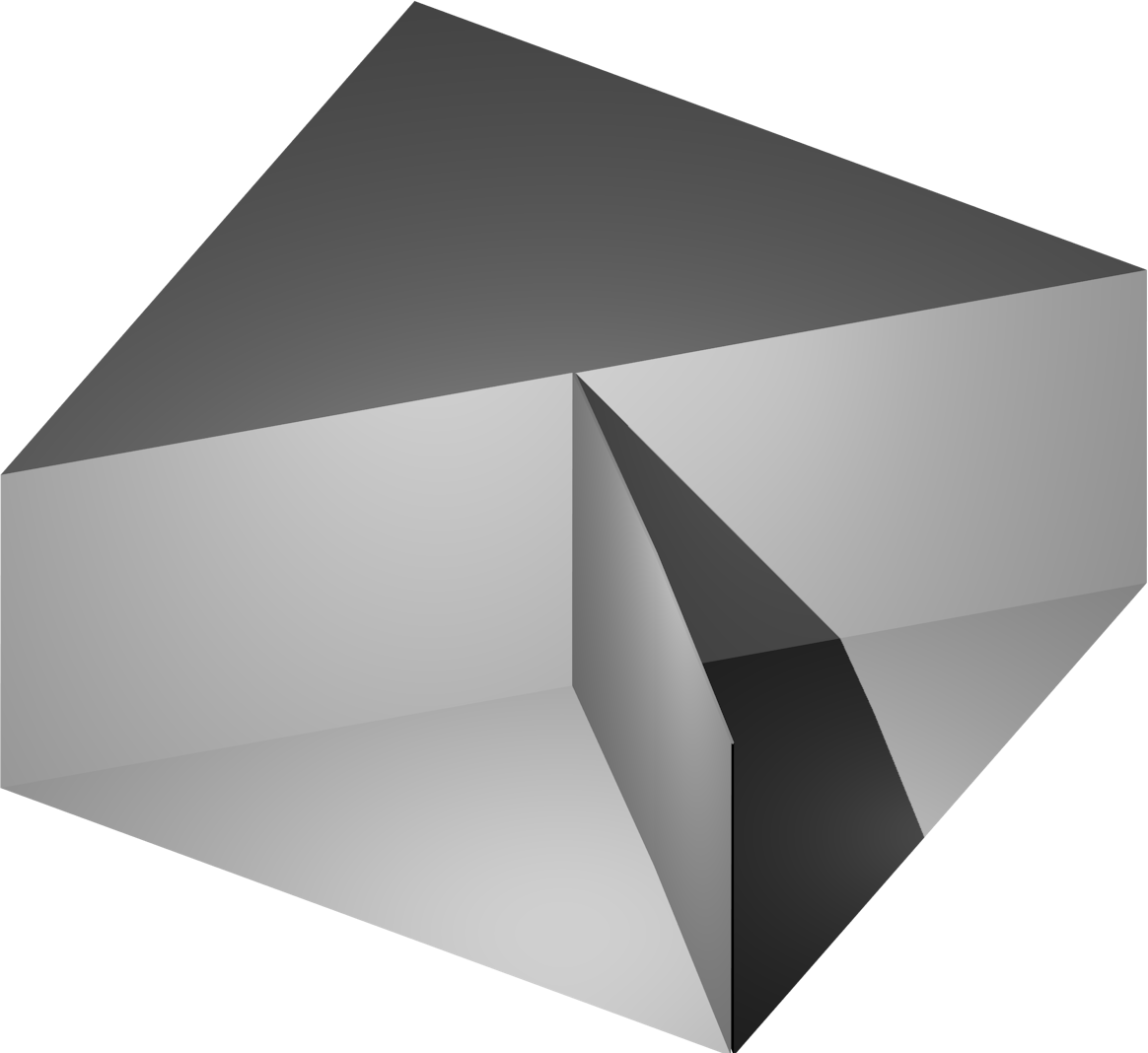
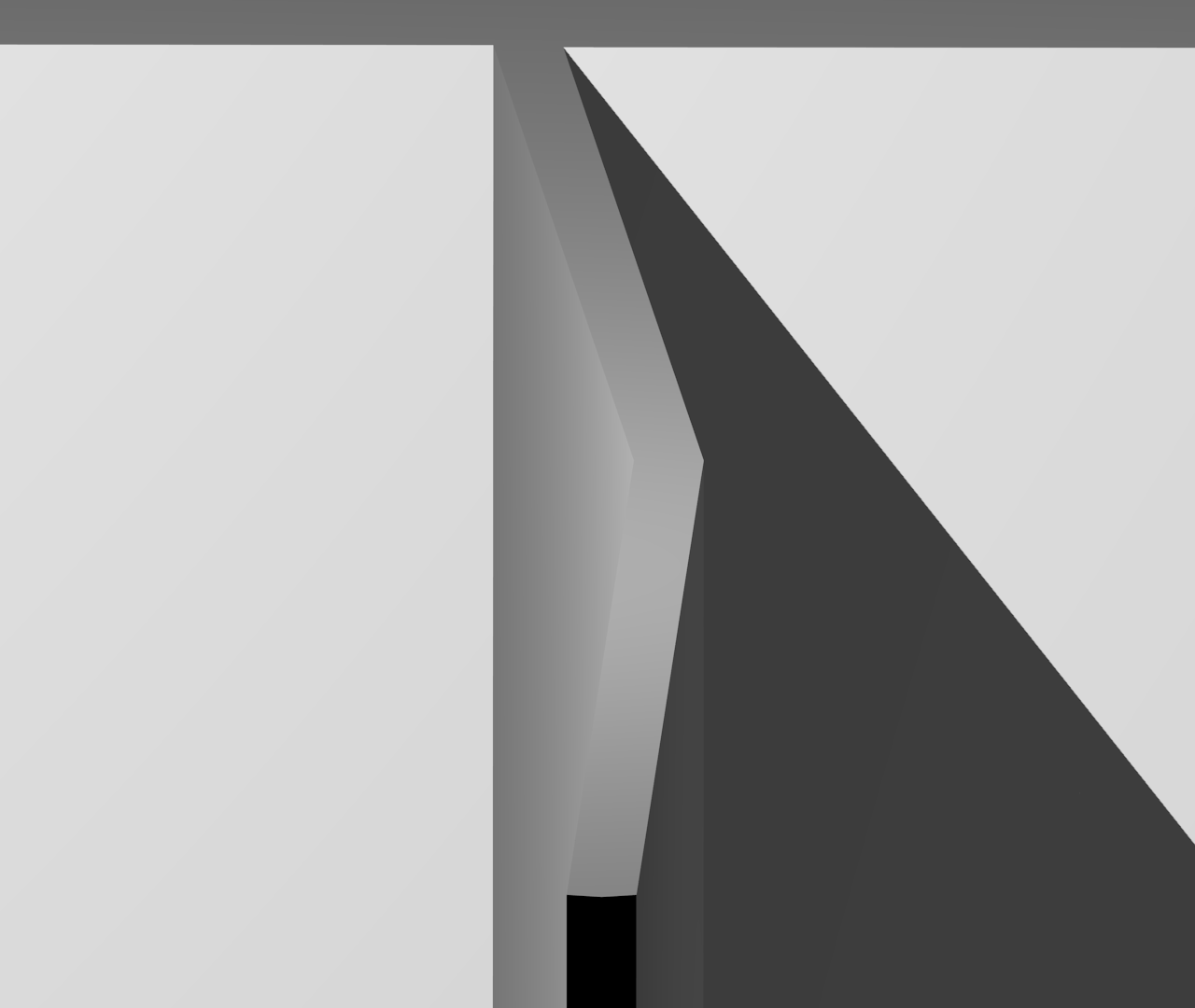
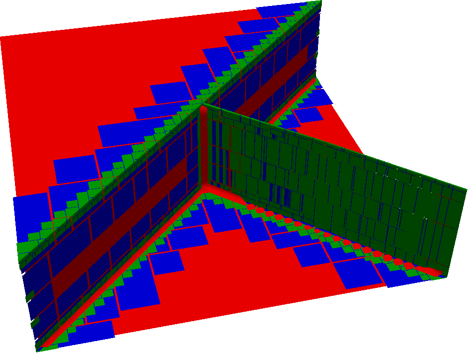
The 3D example consists of (i) a step diagonal through the simulation domain and (ii) a thin trench from the center of the domain to one corner. In Figure 7.4 a rendering of the interface representing the trench is shown from the bottom (viewing it from the top would only show the step and a thin line unable to visually grasp the trench). Note that from the bottom perspective the trench looks like a thin fin instead of a thin trench because the difference between a fin and trench is just the viewpoint. The trench, as in the 2D Trench example, has a width smaller than the spatial resolution of Level 0. Additionally, the trench has a slight dent to avoid an alignment with the computational grid, to provide a more challenging test case. The dent is shown in Figure 7.4b, by a close up on the trench (also shown from the bottom). The example is also inspired by the common high aspect ratio geometries in microelectronic devices [192, 193].

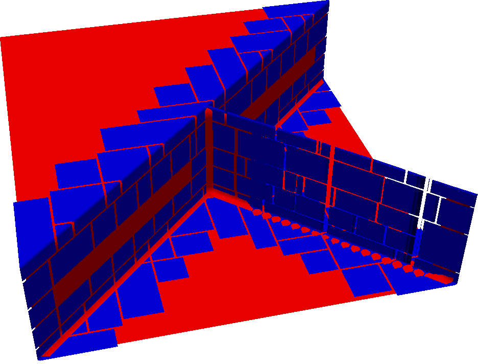
Compared to the 2D examples there are significantly more blocks on Level 1 and Level 2, 107 and 591, respectively. Their placement is visualized in Figure 7.5, by showing their individual contributions to the interface. All blocks on Level 1 have combined $674 496$ grid points and on Level 2 $6 146 688$ grid points.

Accuracy Evaluation

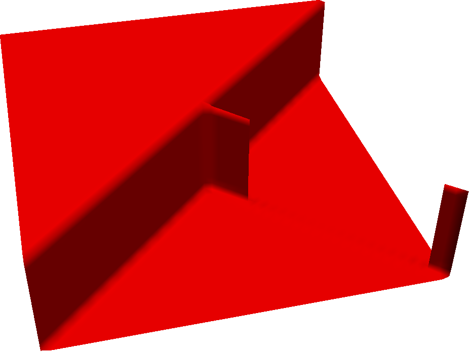
The measured error norms are shown in Table 7.4. On Level 0 the reduction for any error norm is at least a factor of 4.2, because the trench is not resolved on this level (cf. Figure 7.5a, where the extracted interface is based on Level 0 only). The reductions in the error norm on Level 1 are similar to the 2D Trench examples for the $L_{1}$ -norm and $L_{2}$ -norm, due to the same reasons (increased accuracy at rarefaction fans at the bottom of the trench). In contrast, the $L_{\infty}$ -norm for Level 1 is not decreased by applying the bottom-up correction algorithm. The reason for this is that the grid point causing the high $L_{\infty}$ -norm is neither covered directly by a block on the higher level nor in a region where the marching increases the accuracy. Instead, the point is located on a shock wave. The proposed bottom-up correction algorithm is not able to improve the accuracy there. The cause of such errors is that the stencil used for calculating this grid point crosses the skeleton [194, 195]. The skeleton is the union of all shock waves or, equivalently the skeleton is the union of all points which do not have a unique closest point on the interface. In [100] a skeleton aware approach is suggested (but not further investigated here), which might overcome this issue, by adapting the FMM to only consider grid points which are not separated by the skeleton in addition to the upwind direction.

Table 7.4: Error norms for the 3D Trench example, with and without the bottom-up correction algorithm applied, and the corresponding factor by which the error norm is reduced. Adapted with permission from Springer Nature: Springer Cham, Quell et al., Studies in Computational Intelligence 902 (2021), pp. 438-451. [100], © 2021, under exclusive license to Springer Nature Switzerland AG.


Level	$L_{1}$ -norm	L1-reduc.	$L_{2}$ -norm	L2-reduc.	$L_{\infty}$ -norm	inf-reduc.


0	1.853e-2		1.356e-4		4.593e-1
0 corrected	4.422e-3	4.2	2.644e-5	5.1	3.478e-2	13.2
1	2.426e-4		1.259e-6		1.418e-2
1 corrected	1.588e-4	1.5	8.429e-7	1.5	1.418e-2	1.0
2	3.165e-5		7.340e-8		3.017e-3

Performance Evaluation

The 3D Trench example has a high computational load compared to the previously considered 2D examples. This allows to evaluate the performance impact of the bottom-up correction algorithm by measuring the run-time of the top-down re-distancing algorithm and bottom-up correction algorithm on the compute system VSC3. The block-decomposition proposed in Chapter 6 is not employed, because the focus is on the effects of the proposed bottom-up correction algorithm. Figure 7.6 shows the run-time and parallel speedup for the top-down re-distancing algorithm (Re-Distancing), the bottom-up correction algorithm (Correction), and both together (Total) for all three levels of the hierarchical grid combined. For a single thread the run-time introduced by the additional correction algorithm is increased by 4 % and for 16 threads (full utilization of the compute system) by 10 %. The overhead introduced by the by the additional correction algorithm is acceptable, because it allows a proper signed-distance field for thin trenches.

A parallel speedup of 9.3 is achieved with 16 threads for the Re-Distancing with the bottom-up correction algorithm, which is slightly below the parallel speedup for the Re-Distancing without the bottom-up correction algorithm (parallel speedup 9.8). The inferior parallel speedup of 4.1 of the bottom-up correction algorithm alone is caused by the non-parallelized marching on Level 0 (it contains only a single block). Therefore, a level-by-level comparison is necessary to properly evaluate the performance of the bottom-up correction algorithm.

Level-by-Level Comparison

Figure 7.7 shows the level-by-level comparison, except for Level 2, because this is the last level and, as previously mentioned, no correction is performed. The run-time and parallel speedup depend strongly on the level, because the number of blocks and the number of grid points differ significantly.

Starting the investigation on Level 1, the bottom-up correction algorithm has a parallel speedup of 7.5, which is similar to the top-down re-distancing algorithm with a parallel speedup of 7.8. The reason for the slightly reduced parallel speedup is the reduced computational load (not all grid points are re-computed). This leads to a larger overhead of the synchronization tasks. Also, for more than eight threads (fully utilizing one of the two processors of the single utilized node of VSC3) the initialization shows no additional parallel speedup because of NUMA limitations (interpolation between blocks occurs across memory domains).

Finalizing the investigation on Level 0 shows that practically no parallel speedup is observed, because this level only contains a single block. However, the block-decomposition proposed in Chapter 6 solves this issue but is not further considered here. Only the initialization benefits slightly from the additional threads, because the interpolation is parallelized on the blocks on Level 1. The minimum run-time is reached using eight threads. For more than eight threads NUMA effects increase the run-time again.

7.3 Summary

In this chapter a bottom-up correction algorithm for the computational step Re-distancing has been presented. This correction algorithm is tailored towards the FMM and hierarchical grids. The signed-distance field is corrected by interpolation from higher levels of the hierarchical grid and a specialized restarted FMM allows for the bottom-up correction of the signed-distance field even in regions not covered by blocks on higher levels.

The advantageous effect on the accuracy has been evaluated on 2D examples as well on a 3D example. The accuracy of the signed-distance field is significantly increased for a corner by a factor of up to 2.7 (depending on the angel enclosing the corner). In a case where a feature is too small to be represented on a coarse level, i.e., a trench thinner than the grid resolution, the correction algorithm ensures a proper representation. The feature is now represented in the signed-distance field on the coarser level. For the 3D example the impact of the bottom-up correction algorithm on the computational performance has been evaluated, yielding a run-time overhead compared to the top-down re-distancing algorithm presented in Chapter 6 between 4 % and 10 %, which is an acceptable trade off for the proper representation for thin trenches. The evaluation of the parallelization showed a parallel speedup of 9.3 for 16 threads for all levels combined and a similar parallel speedup as for Re-Distancing without the bottom-up correction algorithm for a level-by-level comparison. The block decomposition presented in Chapter 6, may also be employed for the bottom-up correction algorithm to enable a better performance.