Dissertation — Parallel Velocity Extension

Chapter 5 Parallel Velocity Extension

This chapter presents the general details of the computational step Velocity Extension and, in particular, the developed algorithmic advances enabling efficient parallel execution on hierarchical grids.

Velocity Extension extends the given interface velocity (originating from a process model) from the Cross Points (cf. Section 4.2.3, crossings of the grid lines with the interface) to all grid points of the computational domain. Depending on the process model the interface velocity may be a scalar or vector field. The extension is necessary for the level-set equation to be well defined, because a velocity field is required (due to the Eulerian formulation) in the entire computational domain.

First, the analytic requirements to the extended velocity field are precisely defined, which is followed by a literature review of the previous approaches (Section 5.1). The Velocity Extension typically consist of two phases:

The first phase is the extension from the Cross Points to the Close Points (Section 5.2). Cross Points are located directly at the interface and do not belong to the grid. Figure 5.1a schematically shows the Cross Points on which the velocity is given. Close Points are grid points which have a neighboring grid point with a different sign, thus the interface is next to them and as well as at least one Cross Point. Figure 5.1b shows the extension of the velocity from the Cross Points (along the arrows) to the Close Points. This phase is computationally negligible and straightforward parallelizable. The second phase is the extension to the remaining grid points (cf. Figure 5.1c), which is the computationally most intense part.

The extension in the second phase is based on the FMM; the fundamentals of the FMM are presented in detail in Section 5.3. The bottleneck of the FMM is its usage of a heap data structure to sort grid points by their distance to the interface. The sorting determines the order in which the velocity is extended to the grid points. The usage of a heap data structure is inherently serial, because only a single point (the one with the smallest distance) is available for computation.

The core contribution presented in this chapter is to overcome this bottleneck and parallelize the FMM for Velocity Extension. To that end, three advancements were developed and evaluated [56, 137, 138]:

Advancement 1: Through an interpretation of the order of computations in the context of graph theory, it is possible to relax the strict sorting employed by the FMM. This enables the usage of alternative data structures compared to the inherently serial heap employed by the FMM (Section 5.4).

Advancement 2: The change of the data structure allows for a straightforward parallelization of the computations on a Cartesian grid (Section 5.5). The proposed parallelization minimizes the number of explicit synchronization constructs, which favors parallelism. This approach introduces limited redundant computations, i.e., velocity computed on a grid point multiple times. However, the redundancy has negligible negative impact on the parallel performance.

Advancement 3: Finally, the algorithm is tailored to hierarchical grids by a load-balancing approach (Section 5.6). The goal is to reduce global synchronization barriers necessary in the exchange of data between blocks and considerations due to data locality allowing better cache reuse. The different stages of the development of the new algorithm are shown to specifically highlight the advances made and discuss their impact. The performance is evaluated on two representative process TCAD simulations (Section 5.7).

First, an ion beam etching (IBE) simulation, which is part of the fabrication process of a novel device used in memory technology¹ is considered (Section 5.7.1). In this example the scalar velocity extension on a Cartesian grid is analyzed by comparing the run-time of the velocity extension for three different data structures. The parallelization is evaluated by measuring the parallel speedup and the ratio of redundant computations (due to less explicit synchronization constructs).

Second, the thermal oxidation simulation from the motivational example in Section 1.1 is used for analysis, because the process models require the extension of a scalar and a vector velocity (Section 5.7.2). This simulation fully utilizes a hierarchical grid and, therefore, is suited to evaluate the proposed load-balancing and reduced number of global synchronization barriers. The evaluation is performed by measuring the run-time and parallel speedup of the velocity extension step.

¹ The spin-transfer torque magnetoresistive random access memory (STT-MRAM) uses magnetism for permanent storage (without requiring constant supply of electricity, prevalent in current random access memory devices) of information.

5.1 General Ideas

In a semiconductor process TCAD simulation the process model typically provides the interface propagation velocity only for points on the interface. As previously discussed, these points are computationally captured with Cross Points. However, in order to advect the interface the velocities are necessary in the entire computation domain (on the actual grid points). The formal mathematical requirement to an extended velocity field is that it is continuous in regions close to the interface, i.e.:

$\begin{matrix} (5.1) & lim_{\vec{x} \to Γ} V = V_{I} . \end{matrix}$

The continuity is achieved in practice by assigning each point the velocity of the closest point on the interface. The velocity extension equation

$\begin{matrix} (5.2) & \nabla Φ (\vec{x}, t) \cdot \nabla V (\vec{x}, t) = 0, \end{matrix}$

is used to describe this. In case of a signed-distance field $Φ$ it is equivalent to constantly extend the velocity along interface normal vectors. Additionally, an extension according to (4.19) avoids distortions of the signed-distance field (still distortions occur due to numeric errors). This fact was first proven in [122] and follows:

$\begin{aligned} \frac{d | \nabla Φ (\vec{x}, t) |^{2}}{d t} & = \frac{d}{d t} (\nabla Φ (\vec{x}, t) \cdot \nabla Φ (\vec{x}, t)) \\ = 2 \nabla Φ (\vec{x}, t) \cdot \frac{d}{d t} \nabla Φ (\vec{x}, t) \\ = - 2 \nabla Φ (\vec{x}, t) \cdot \nabla V_{} | \nabla Φ (\vec{x}, t) | - 2 \nabla Φ (\vec{x}, t) \cdot \nabla | \nabla Φ (\vec{x}, t) | V_{} . \end{aligned}$ For a signed-distance function ( $| \nabla Φ (\vec{x}, t = 0) | = 1$ ), $Φ$ stays a signed-distance function. The changes to the last line result from swapping the time and spatial derivative and using the level-set equation (4.9). The first term is zero because of the choice for the extended velocity (4.19). The second term is zero due to starting with a signed-distance function (gradient of a constant function is zero). In case of a vector-valued velocity field (4.19) is solved for each component of the vector velocity as in the scalar case.

The investigation starts with a review of approaches to solve the velocity extension problem.

Literature Review

There are several strategies to solve the velocity extension problem, considering only the basic case of a Cartesian grid. The first attempt was made in [122] using the FMM which is based on Dijkstra’s algorithm [139]. The FMM traverses the grid points of the computational domain using a priority queue in ascending order visiting every grid point exactly once. The computational complexity of this approach is $O (n \log (n))$ with $n$ the number of grid points in the computational domain, due to the necessary sorting of the priority queue (cf. Section 5.3).

In [140] the approach is further developed to yield higher accuracy for characteristic curves² at the cost of higher computational load. The higher accuracy is especially important, if the velocity field shall be used for several time steps of a simulation (reducing the number of evaluations of the process model), i.e., evaluating the process model only every third time step. This is not used in the presented level-set simulations, because the underlying velocities from the process model can change significantly between two consecutive time steps.

In [141] an approach based on the fast scanning method is introduced. It iteratively computes the velocity on all grid points of the computational domain using several predefined stencil configurations. The run-time complexity is $O (n)$ with $n$ the number of grid points in the computational domain. A drawback is that the approach visits every grid point of the computational domain $2^{d}$ times, with $d$ the number of spatial dimensions.

The velocity extension presented in [142] allows for faster convergence for shape optimization simulations based on the level-set method, i.e., minimizing the volume of a cantilever but maintaining a certain resistance to deformation. This approach is not applicable to process TCAD simulations, because it requires an already established velocity field for one side of the interface: In process TCAD simulations, the velocity field is only available at the Cross Points directly at the interface.

An approach based on the biharmonic expansion is presented in [143], but is not applicable because an already established velocity field for one side of the interface is required. The same issue applies to the extrapolation approach based on fast sweeping methods presented in [144].

In [145] an extension based on solving local Riemann problems is proposed. This approach achieves a higher simulation accuracy compared to an approach based on the FMM. For small time steps the asymptotic limit of the extension based on local Riemann problems and the FMM are the same. Thus the simulation results are also the same.

However, approaches for efficient parallelization of the velocity extension are missing, in particular when considering hierarchical grids.

² A curve describing the movement of a point driven by a PDE.

5.2 Extension from Cross Points to Close Points

The first step for all reviewed velocity extension algorithms (which are applicable to the process TCAD simulation setting) is to extend the velocity from Cross Points to the Close Points.

Let $d_{x}, d_{y},$ and $d_{z}$ be the distances from a Close Point to the Cross Points in $x$ -dimension, $y$ -dimension, and $z$ -dimension, respectively. The gradient of $Φ$ computed at the Close Point via first-order finite differences to the Cross Points is given by

$\begin{matrix} (5.3) & (\frac{d}{d_{x}}, \frac{d}{d_{y}}, \frac{d}{d_{z}}), \end{matrix}$

with $d$ the distance to the interface of the Close Point ( $Φ$ value).

The velocity at the Cross Points is $v_{x}, v_{y},$ and $v_{z}$ . Inserting the finite difference approximations to the gradients into the velocity extension equation (4.19) yields

$\begin{aligned} 0 & = (\frac{v - v_{x}}{d_{x}}, \frac{v - v_{y}}{d_{y}}, \frac{v - v_{z}}{d_{z}}) \cdot (\frac{d}{d_{x}}, \frac{d}{d_{y}}, \frac{d}{d_{z}}) \\ = d (\frac{v - v_{x}}{d_{x}^{2}} + \frac{v - v_{y}}{d_{y}^{2}} + \frac{v - v_{z}}{d_{z}^{2}}) . \end{aligned}$ Solving for $v$ gives

$\begin{matrix} (5.4) & v = \frac{d_{y}^{2} d_{z}^{2} v_{x} + d_{x}^{2} d_{z}^{2} v_{y} + d_{x}^{2} d_{y}^{2} v_{z}}{d_{x}^{2} d_{y}^{2} + d_{x}^{2} d_{z}^{2} + d_{y}^{2} d_{z}^{2}} . \end{matrix}$

Thus the velocity on the Close Points is given as the weighted average of the velocity of the closest Cross Point in each spatial dimension.

In case no Cross Point is available for a specific spatial dimension (5.4) a lower dimensional computation is performed, e.g., if in $z$ -dimension no Cross Point is available, the formula is simplified to

$\begin{matrix} (5.5) & v = \frac{d_{y}^{2} v_{x} + d_{x}^{2} v_{y}}{d_{x}^{2} + d_{y}^{2}} . \end{matrix}$

Figure 5.2 shows the variables denoted above for the 2D case.

Figure 5.2: The velocity

v

of a Close Point (red) is computed using the velocities from the Cross Points (blue). The Cross Point (green) is ignored as a closer Cross Point in the

x

-dimension is available.

If a Cross Point is only available in a single spatial dimension, e.g., $x$ -dimension, no computation is necessary as the velocity from the Cross Point is directly assigned

$\begin{matrix} (5.6) & v = v_{x} . \end{matrix}$

The distance $d$ of the Close Point is not used in the computation of $v$ and only the velocities from Cross Points are used. The velocity is computed independently for all Close Points, thus allowing for a straightforward parallelization of the extension to the Close Points.

Now that the velocity is available for all Close Points, the FMM is used to extend the velocity to the remaining grid points (computational domain). Due to the data dependencies between the grid points this is more complicated than the above discussed extension from Cross Points to Close Point and an ordering scheme is required.

5.3 Fast Marching Method

The FMM assigns each grid point of the computational domain one of three exclusive flags (states):

• Known: The grid point has its final velocity (value) assigned and no further updates are necessary.
• Band: The grid point has a temporary velocity (value) assigned (the velocity might be changed by a subsequent update).
• Unknown: The grid point has no velocity (value) assigned.

Based on these flags the FMM for the velocity extension is described as it is presented in [122]. First, a set of initial grid points is chosen around the interface (Close Points), and afterwards the velocity is extended to neighboring grid points by solving the discretized version of (4.19) using an upwind scheme. This allows to compute the solution in a from the interface outwards marching manner.

The computation of the velocity on a grid point is described in Algorithm 1. It is similar to the computation used for the extension from the Cross Points to the Close Points, but now all involved points are part of the grid. First, the upwind neighbors are determined in each spatial dimension (neighboring grid points with a smaller distance to the interface). The $Φ$ values of the neighboring grid points are compared based on considering three cases: In case the lower neighboring grid point (neighboring grid point with the smaller index) is selected (cf. Algorithm 1 Line: 5), in case the higher neighboring grid point (neighboring grid point with a larger index) is selected (cf. Algorithm 1 Line: 9), and in case none is selected the contribution from this spatial dimension is zero, subsequently ignored. The selected neighbors are then used in the approximation to the gradient by computing the forward/backward differences. Finally, the weighted average of the velocities is computed (Algorithm 1 Line: 14) and the grid point is flagged Band (Algorithm 1 Line: 15).

1 procedure Update( $P$ ):

/* Determine upwind neighbors of $P$ */

2 for $i \in {x, y, z}$ do

3 $D_{i} \leftarrow 0$

4 $V_{i} \leftarrow 0$

5 if $P^{- i} . Φ < P^{+ i} . Φ$ and $P^{- i} . Φ < P . Φ$ then

6 $D_{i} \leftarrow \frac{P . Φ - P^{- i} . Φ}{Δ_{i}^{2}}$

7 $V_{i} \leftarrow P^{- i} . V$

8 end if

9 if $P^{- i} . Φ > P^{+ i} . Φ$ and $P^{+ i} . Φ < P . Φ$ then

10 $D_{i} \leftarrow \frac{P . Φ - P^{+ i} . Φ}{Δ_{i}^{2}}$

11 $V_{i} \leftarrow P^{+ i} . V$

12 end if

13 end for

/* Compute velocity for $P$ according to the upwind scheme */

14 $P . V \leftarrow \frac{\sum_{i \in {x, y, z}} V_{i} D_{i}}{\sum_{i \in {x, y, z}} D_{i}}$

15 $P .$ flag $\leftarrow$ Band

16 end procedure

Algorithm 1: Procedure to update (compute) the velocity on the given grid point $P$ . First, the upwind neighbors of P are determined and then the weighted average of their velocities is computed and the flag is set to Band.

The computation of the velocity on a grid point is illustrated by a small example.

Example

In order to illustrate the update of a grid point $P$ with its index $i j k$ , the following specific configuration is considered. In $x$ -dimension the lower neighboring grid point ( $P^{- x}$ with index $i - 1 j k$ ) is closer to the interface, as well as in the $y$ -dimension ( $P^{- y}$ with index $i j - 1 k$ ), but in the $z$ -dimension none of the neighboring grid points is closer to the interface, thus the used first-order upwind scheme is given by

$\begin{array}{r} (5.7) & 0 = (\frac{V_{i - 1 j k} - V_{i j k}}{Δ_{x}}, \frac{V_{i j - 1 k} - V_{i j k}}{Δ_{y}}, 0) \cdot (\frac{Φ_{i - 1 j k} - Φ_{i j k}}{Δ_{x}}, \frac{Φ_{i j - 1 k} - Φ_{i j k}}{Δ_{y}}, 0) . \end{array}$ Solving for the velocity in this case yields

$\begin{array}{r} (5.8) & V_{i j k} = \frac{V_{i - 1 j k} \frac{Φ_{i - 1 j k} - Φ_{i j k}}{Δ_{x}^{2}} + V_{i j - 1 k} \frac{Φ_{i j - 1 k} - Φ_{i j k}}{Δ_{y}^{2}}}{\frac{Φ_{i - 1 j k} - Φ_{i j k}}{Δ_{x}^{2}} + \frac{Φ_{i j - 1 k} - Φ_{i j k}}{Δ_{y}^{2}}} . \end{array}$ In case the grid resolution is the same for all spatial dimensions $Δ_{x} = Δ_{y} = Δ_{z}$ , the dependency of the solution on the grid resolution vanishes yielding

$\begin{array}{r} (5.9) & V_{i j k} = \frac{V_{i - 1 j k} (Φ_{i - 1 j k} - Φ_{i j k}) + V_{i j - 1 k} (Φ_{i j - 1 k} - Φ_{i j k})}{Φ_{i - 1 j k} - Φ_{i j k} + Φ_{i j - 1 k} - Φ_{i j k}} . \end{array}$

The detailed discussion of the FMM as shown in Algorithm 2 follows.

FMM Algorithm

The FMM is initialized by first flagging all grid points Unknown (Algorithm 2 Line: 3) and then the velocity on all the Close Points is computed and they are flagged Known (Algorithm 2 Line: 7). The next step is to advance to all the neighboring grid points of the Close Points and compute their velocity and set their flag to Band. The computation of the velocity on a neighboring grid point is performed using Algorithm 1.

1 procedure FastMarchingMethod():

/* Initialization - Grid points and Band */

2 foreach grid point [P] do // Initialize all grid points

3 P.flag $\leftarrow$ Unknown

4 end foreach

5 foreach Close Points [CP] do

6 CP.V $\leftarrow$ Velocity computed based on the Cross Points

7 CP.flag $\leftarrow$ Known

8 end foreach

9 foreach Close Points [CP] do // Setup the priority queue

10 foreach CP.Neighbors [N] do

11 if N.flag = Unknown then

12 Update(N)

13 end if

14 end foreach

15 end foreach

/* Marching - Extend to the computational domain */

16 while Band $\neq \emptyset$ do

17 P $\leftarrow min$ Band // Main challenge for parallelization

18 P.flag $\leftarrow$ Known

19 foreach P.Neighbors [N] do

20 if N.flag = Unknown then

21 Update(N)

22 end if

23 end foreach

24 end while

25 end procedure

Algorithm 2: The FMM used on a Cartesian grid for the velocity extension.

The key idea of the FMM is that from all the grid points flagged Band the one with the smallest distance to the interface is chosen and flagged Known (Algorithm 2 Line: 17). This guarantees that for the immediately following update of all neighboring grid points (Algorithm 2 Line: 21) the velocities on grid points used in Algorithm 1 are already computed beforehand. The updated neighboring grid points are flagged Band, thus they are also considered when the next grid point is chosen to be flagged Known.

The step selecting the grid point flagged Band with the smallest distance to the interface is repeated until no more grid point is flagged Band, thus all grid points are flagged Known. The first part of Algorithm 2, in particular Lines: 2-15, is typically referred to as initialization of the FMM, because it sets the stage for the second part, the marching, in particular Algorithm 2 Lines: 16-24. The term marching originates from the Eikonal equation (Section 6.1), where the solution process corresponds to a front marching away from an interface.

The efficient selection of the minimum in Algorithm 2 Line: 17 is key to the performance of the FMM, which is discussed in the next section.

5.4 Data Structures

For an efficient selection of the grid point (also flagged Band) with the smallest distance to the interface all Band grid points are ordered by their distance to the interface, which is implemented by a priority queue. To efficiently sort the grid points in a priority queue a specialized data structure is employed. Typically a heap data structure (Heap) is used [122, 67, 146]. From the available heap data structures the binary heap (in form of a binary tree) is the most used implementation. The data structure has to provide the following functionality:

• getFirst shall return the first point (for the FMM the first point is the one with the smallest distance to the interface) and remove it from the data structure.
• insert shall insert a grid point into the data structure. In case of a Heap insert additionally verifies that no grid point is inserted twice, because, if a grid point is already present in the Heap, only the position within the heap is updated.

Figure 5.3 depicts the insert and getFirst operations. The insert operation appends the new element to the binary tree (last position). Afterwards, the element bubbles up (is swapped with its parent) until its current parent is smaller. The getFirst operation removes the smallest element and puts the last element in the binary tree on its position. Afterwards, the last element (now on the first place) bubbles down (is swapped with its children) until its current parent is smaller. Thus, both operations require the swapping of several other elements of the heap to ensure the correct ordering of the elements in the heap.

Inserting a grid point to the binary heap and removing the first grid point has the computational complexity of $O (\log (n))$ . Removing the first grid point also has the computational complexity of $O (\log (n))$ . In both cases several swaps are necessary to keep the heap in order. Consequently, the FMM has a computational complexity of $O (n \log (n))$ , because all $n$ grid points of the computational domain have to be inserted into and removed from the binary heap. The usage of a priority queue in form of a Heap is counterproductive for parallelization, because only the single element with the smallest key (distance to the interface) is eligible for an update. The goal of the next paragraphs is to lay out the developed approach of relaxing the strict ordering enforced by the binary heap to (i) enable a computational complexity of $O (n)$ and (ii) to enable parallelization of the algorithm.

Graph Theory

To relax the ordering enforced by the FMM, the problem is interpreted in the context of graph theory. Let $G (N, E)$ be an ordered graph, where the nodes $N$ are given by all the grid points and the edges $E$ are given by the upwind neighbor relationship. Figure 5.4 shows an exemplary graphical representation of such a graph. The graph is divided into two independent partitions through the interface (inside and outside). For simplicity’s sake only one of those partitions is considered here, because the exact same algorithm is applied to the other partition. This enables a straightforward parallelization for up to two threads processing both sides of the interface simultaneously.

The order in which the nodes are able to be computed is equivalent to the topological sort problem, which is possible to be solved in linear $O (| N | + | E |)$ time as shown in [147]. Topological sort of a directed graph is a linear ordering of its nodes such that every edge is directed the same, i.e., consider all nodes to be placed on a straight line and all edges point to the right. The topological order of a graph is not unique, if there is more than one source which is a node with no incoming edge, i.e., in the context of the velocity extension all the Close Points are sources.

The computational complexity is also linear in the number of grid points in the computational domain, because $n = | N |$ and the number of edges $| E |$ in the graph is limited by the used stencil to approximate the gradients. The typically used stencil contains the direct neighbors only, thus $| E | \leq 2 d | N |$ with $d$ the number of spatial dimensions. For example, in three spatial dimensions the seven-point stencil yields $| E | \leq 6 | N |$ . Comparing the newly developed approach which requires in the worst case only $2 d$ visits of each grid point, to the fast scanning method approach which requires always $2^{d}$ visits, shows the advantage.

The topological sort problem is typically solved by a depth-first or breadth-first traversal of the graph [148]. A depth-first traversal moves along an edge to the next node before it returns to explore the other edges of a node. A breadth-first traversal explores first all edges of a node before it moves to the next node.

Those algorithms can be adapted to the FMM based approach, as they influence the ordering of the grid points in the Band. Using a Stack (first-in last-out queue, Figure 5.5a) corresponds to a depth-first and using a Queue (first-in first-out queue, Figure 5.5b) corresponds to a breadth-first traversal, respectively. The classic FMM uses a Heap (binary heap) data structure. Figure 5.5 shows graphically that insert and getFirst are less complex for the Stack and Queue compared to the Heap (cf. Figure 5.3). The binary heap data structure performs insert and getFirst operations in $O (\log (n))$ , whilst the Stack and Queue data structure perform those operations in $O (1)$ .

The necessary changes to the algorithms are presented and discussed in the next paragraphs.

Algorithmic Changes

The adaptions necessary to the FMM are shown in Algorithm 3 and the changes to the Update algorithm are shown in Algorithm 4, which is extended compared to Algorithm 1. A check whether the grid point is already computed Algorithm 4 Line: 2 is added, because for a Stack and Queue a grid point might be inserted multiple times into the data structure of the Band. Also, a check whether all upwind neighbors have already a velocity assigned is necessary (Algorithm 4 Line: 9 and Algorithm 4 Line: 16). Only the ordering of the computations by the Heap guarantees that all upwind neighbors are computed beforehand. If not all upwind neighbors have already a velocity assigned (one of them is flagged Unknown) then the velocity is not computed. The grid point is again considered when the previously Unknown upwind neighbor is computed and, therefore, it is guaranteed that all grid points are computed when the algorithm terminates.

1 procedure Velocity Extension():

/* Initialization - Grid points and Band */

2 foreach Points [P] do // Initialize all grid points

3 P.flag $\leftarrow$ Unknown

4 end foreach

5 foreach Close Points [CP] do

6 CP.velocity $\leftarrow$ Velocity computed based on the Cross Points

7 CP.flag $\leftarrow$ Known

8 end foreach

9 foreach Close Points [CP] do // Setup the priority queue/queue/stack

10 foreach CP.Neighbors [N] do

11 if N.flag = Unknown then

12 Update2(N)

13 end if

14 end foreach

15 end foreach

/* Marching - Extend to the computational domain */

16 while Band $\neq \emptyset$ do

17 P $\leftarrow$ getFirst Band // first (instead of smallest) grid point is chosen

18 P.flag $\leftarrow$ Known

19 foreach P.Neighbors [N] do

20 if N.flag = Unknown then

21 Update2(N)

22 end if

23 end foreach

24 end while

25 end procedure

Algorithm 3: First modification of the FMM (now just called Velocity Extension), which enables the usage of different data structures for the Band. The Update algorithm is also changed to use the modified algorithm Update2. The blue colored lines are added/modified compared to Algorithm 2.

1 procedure Update2( $P$ ):

2 if $P .$ flag != Unknown then // Skip if already computed

3 return

4 end if

/* Determine upwind neighbors of $P$ and their flag */

5 for $i \in {x, y, z}$ do

6 $D_{i} \leftarrow 0$

7 $V_{i} \leftarrow 0$

8 if $P^{- i} . Φ < P^{+ i} . Φ$ and $P^{- i} . Φ < P . Φ$ then

9 if $P^{- i} .$ flag = Unknown then

10 return // No update takes place

11 end if

12 $D_{i} \leftarrow \frac{P . Φ - P^{- i} . Φ}{Δ_{i}^{2}}$

13 $V_{i} \leftarrow P^{- i} . V$

14 end if

15 if $P^{- i} . Φ > P^{+ i} . Φ$ and $P^{+ i} . Φ < P . Φ$ then

16 if $P^{+ i} .$ flag = Unknown then

17 return // No update takes place

18 end if

19 $D_{i} \leftarrow \frac{P . Φ - P^{+ i} . Φ}{Δ_{i}^{2}}$

20 $V_{i} \leftarrow P^{+ i} . V$

21 end if

22 end for

/* Compute velocity for $P$ according to the upwind scheme */

23 $P . V \leftarrow \frac{\sum_{i \in {x, y, z}} V_{i} D_{i}}{\sum_{i \in {x, y, z}} D_{i}}$

24 $P .$ flag $\leftarrow$ Band

25 end procedure

Algorithm 4: Procedure to update (compute) the velocity on the given grid point $P$ , with additional checks compared to Algorithm 1 (blue colored lines). The checks ensure that the velocity is computed on the upwind neighbors.

The impact of the different data structures on the performance is evaluated in Section 5.7.1, however, first the parallelization of the Velocity Extension is discussed.

5.5 Parallelization

The relaxation of the strict ordering of the FMM allows for a parallelization of the velocity extension algorithm, which is shown in Algorithm 5. The for-loops in Algorithm 5 Line: 2 and Line: 5 are straightforward parallelizable as all the iterations are independent.

1 procedure Velocity Extension Parallel():

/* Initialization - Grid points */

2 foreach Points [ $P$ ] do // In parallel

3 $P .$ flag $\leftarrow$ Unknown // Initialize all grid points

4 end foreach

5 foreach Close Points [ $C P$ ] do // In parallel

6 $C P .$ velocity $\leftarrow$ Velocity computed based on the Cross Points

7 $C P .$ flag $\leftarrow$ Known

8 end foreach

/* Marching - Extend to the computational domain */

9 foreach Close Points [ $C P$ ] do // In parallel

10 create WQ

11 WQ.insert( $C P$ )

12 while WQ $\neq \emptyset$ do // Extend velocity to entire domain

13 $P$ $\leftarrow$ WQ.getFirst

14 foreach Neighbors [ $N$ ] of $P$ do

15 if $N .$ flag = Unknown then

16 if Update3( $N$ ) then

17 WQ.insert( $N$ )

18 end if

19 end if

20 end foreach

21 end while

22 end foreach

23 end procedure

Algorithm 5: Parallelized velocity extension, by creating an independent work queue (WQ) for each Close Point, allowing for parallel computations.

A single data structure storing the grid points flagged Band is not viable due to the synchronization overhead, if all threads would operate on the same data structure. Thus, for every Close Point a dedicated data structure called WQ is created (Algorithm 5 Line: 10). The WQ is a data structure that supports the insert and getFirst operations. As the WQs track all the grid points flagged Band the explicit label Band is not required anymore and only Known and Unknown are used. Therefore, the initialization of the Band grid points is modified and the Close Points are directly used for the WQ (Algorithm 5 Line: 11). The WQ data structure is exclusive (in OpenMP terms: private) to the executing thread. The block where all grid points (with their velocity and flag) are stored is shared between all the threads.

In principle, explicit synchronization between the threads would be necessary every time a grid point from the shared block is accessed. This is not required for correctness of the velocity extension, but to avoid redundant computations, i.e., two threads compute the velocity simultaneously for the same grid point. That being said, Algorithm 5 deliberately re-computes the velocities, as the computational overhead is negligible compared to an otherwise introduced synchronization overhead. Both threads compute the identical velocity as the upwind grid points and their velocity value used for the computations are the same. Access of a thread to a grid point is required to be an atomic operation for read and write operations. Atomicity is needed to ensure that values are read/written in a consistent manner. Otherwise, writing identical values by two threads to the same grid point might corrupt the data. The changes to Algorithm 5 also require changes to the update algorithm shown in the next paragraph.

Final Update Algorithm

Also the Update2 algorithm is modified yielding the final version of the Update3 algorithm Algorithm 6. The algorithm returns a Boolean indicating whether the update has been successful. The update is not successful, if the grid point is already computed Algorithm 6 Line: 2, or any upwind neighbor is not computed beforehand (Algorithm 6 Line: 9 and Algorithm 6 Line: 16). After the computation of the velocity an additional check is introduced whether the grid point has not been computed in the meanwhile by a different thread (Algorithm 6 Line: 25). This check is not explicitly synchronized with other threads, but reduces redundant computations, especially the otherwise following redundant insertion into the WQ is avoided. To completely avoid the redundant computations an explicit locking mechanism could be considered in principle, however, such an approach would seriously deteriorate the performance.

1 procedure Update3( $P$ ):

2 if $P .$ flag != Unknown then // Computed by another thread

3 return false

4 end if

/* Determine upwind neighbors of $P$ and their flag */

5 for $i \in {x, y, z}$ do

6 $D_{i} \leftarrow 0$

7 $V_{i} \leftarrow 0$

8 if $P^{- i} . Φ < P^{+ i} . Φ$ and $P^{- i} . Φ < P . Φ$ then

9 if $P^{- i} .$ flag = Unknown then

10 return false // No update takes place

11 end if

12 $D_{i} \leftarrow \frac{P . Φ - P^{- i} . Φ}{Δ_{i}^{2}}$

13 $V_{i} \leftarrow P^{- i} . V$

14 end if

15 if $P^{- i} . Φ > P^{+ i} . Φ$ and $P^{+ i} . Φ < P . Φ$ then

16 if $P^{+ i} .$ flag = Unknown then

17 return false // No update takes place

18 end if

19 $D_{i} \leftarrow \frac{P . Φ - P^{+ i} . Φ}{Δ_{i}^{2}}$

20 $V_{i} \leftarrow P^{+ i} . V$

21 end if

22 end for

/* Compute velocity for $P$ according upwind scheme */

23 $P . V \leftarrow \frac{\sum_{i \in {x, y, z}} V_{i} D_{i}}{\sum_{i \in {x, y, z}} D_{i}}$

24 $P .$ flag $\leftarrow$ Band

25 if $P .$ flag != Unknown then // Redundant computation

26 return false

27 else

28 $P . V \leftarrow$ V

29 $P .$ flag $\leftarrow$ Known

30 return true

31 end if

32 end procedure

Algorithm 6: Final procedure to update (compute) the velocity on the given grid point $P$ , with additional checks and a Boolean return value compared to Algorithm 4, to reduce the redundant computations introduced by the parallelization.

Only if the update is successful (Algorithm 6 returns true), the grid point is inserted into the WQ (Algorithm 5 Line: 17). The algorithm terminates if all WQs are empty, meaning all grid points have a velocity assigned.

Explanatory Example

To better illustrate the process of the newly developed algorithm an explanatory example is discussed in the following. In Figure 5.6 an example for a parallel execution of Algorithm 5 is shown using three threads. Three threads work in parallel on the grid. The work completed by a thread is shown by the corresponding color (red, green, blue). For this example it is assumed that each thread processes one node (grid point) per step and is able to handle all neighbors. The edges (arrows) to the neighbor are also colored using the thread color. The arrows are filled, if the neighbor is successfully computed and inserted into a thread’s own WQ. In the first step, each thread has a single WQ containing a single Close Point assigned (marked with a white one in Figure 5.6a). The number on a node indicates the step in which a node has been processed. If the WQ is empty a new WQ is assigned, by selecting a new Close Point, e.g., for the blue thread this happens at step two (Figure 5.6b) and for the green one at step three (Figure 5.6c).

Threads require different numbers of steps to finish, i.e., the green thread requires nine steps whilst the blue thread requires 16 (Figure 5.6d). The green thread is finished (out of work), because no more Close Points (WQs) are available to be processed. This is a typical load-imbalance problem. The cause of this load-imbalance is found in the structure of the given dependencies of the grid points. The longest dependency chain is 10 grid points long. In practical applications, however, the load-imbalance is negligible due to the several orders of magnitude higher number of Close Points compared to the number of used threads.

The developed parallelization approach is evaluated in Section 5.7.1, on a Cartesian grid³. The next section discusses adaptions of the parallel velocity extension step to support hierarchical grids.

³ In the context of hierarchical grids, this is equivalent to a hierarchical grid containing only a single level, hence, also only a single block.

5.6 Hierarchical Grids

In the previous sections the velocity extension has been discussed within the context of a single resolution Cartesian grid. This section extends the algorithms to be used on hierarchical grids.

The hierarchical algorithm is given in Algorithm 7. The developed advancements relative to the previously developed multi-block FMM [62] are highlighted.

1 procedure Extension Hierarchical():

2 setBoundaryConditionsOnLevel 0()

3 foreach Levels do // From coarsest to finest

4 foreach Blocks on Level do // Parallel region

5 WQ $\leftarrow$ InitialPoints // Create task

6 Velocity Extension(Blocks,WQ)

7 end foreach

8 Wait // Synchronization barrier

9 WQ $\leftarrow$ Exchanged ghost points

10 while WQ $\neq \emptyset$ do

11 foreach Blocks on Level do // Parallel region

12 Velocity Extension(Blocks,WQ) // Create task

13 end foreach

14 Wait // Synchronization barrier

15 WQ $\leftarrow$ Exchanged ghost points

16 end while

17 setBoundaryConditionsOnNextLevel()

18 end foreach

19 end procedure

Algorithm 7: The velocity extension algorithm tailored towards a hierarchical grid, the changes colored in red are lines which are removed in comparison to the multi-block FMM.

Algorithm 7 operates in a top-down manner, starting the extension on Level 0 (the coarsest level) and successively extending the velocity on finer (higher) levels. The algorithm also explicitly sets the boundary conditions (cf. Algorithm 7 Line: 2 and Algorithm 7 Line: 17) by involving ghost points. Previous presented algorithms operating on a Cartesian grid ignored the boundary conditions for reasons of a more accessible presentation, but in case of a hierarchical grid setting this it not possible. Ghost points are either set via linear interpolation of the velocity from a coarser level or, if they are covered by a block on the same level, by a non-ghost point of the respective block.

After the boundary conditions are set, for each block on a level a parallel OpenMP task (cf. Section 3.1) is created, allowing the computation of blocks on the same level in parallel (Algorithm 7 Line: 4). Each task creates a dedicated WQ using the Queue as underlying data structure. The union of the Close Points and ghost points for which the velocity is known (InitialPoints) is inserted into the WQ. Subsequently, Algorithm 8 is executed, which extends the velocity based on the given WQ to the corresponding block. After that a global synchronization barrier is enforced, waiting for all tasks to be finished before proceeding as otherwise some ghost points are possibly exchanged before their velocity is computed. Global synchronization barriers are detrimental to parallel performance, because they require all threads to synchronize. This causes threads to idle until the last thread reaches the synchronization barrier. Thus it is desirable to avoid global barriers as proposed in the next paragraphs.

Reducing Global Synchronization

The former multi-block FMM [62] algorithm uses a synchronized exchange step. The synchronized exchange step internally uses two global synchronization barriers. In between the global synchronization barriers the ghost points of all blocks are updated. The here proposed advanced algorithm does not need those synchronized exchange steps anymore because the functionality was transferred into Algorithm 8. This reduces the number of global synchronization barriers, except for one at the end of each processed level. If the velocity for a ghost point is changed by the synchronized exchange step, the ghost point is inserted into the WQ of the corresponding block (Algorithm 7 Line: 9). As long as there is a non-empty WQ, Algorithm 8 is executed again with the same synchronization barrier and synchronized exchange step.

1 procedure Velocity Extension(Block, WQ):

2 foreach Points [P] do

3 P.flag $\leftarrow$ Unknown // Initialize all grid points

4 end foreach

5 foreach Close Points [CP] do

6 CP.velocity $\leftarrow$ Velocity computed based on the Cross Points

7 CP.flag $\leftarrow$ Known

8 end foreach

9 while WQ $\neq \emptyset$ do

10 if WQ.length $>$ limit then

11 WQ $_{1}$ ,WQ $_{2}$ $\leftarrow$ Split WQ

12 Velocity Extension(Block, WQ $_{1}$ ) // Create Task

13 WQ $\leftarrow$ WQ $_{2}$

14 end if

15 P $\leftarrow$ WQ.getFirst()

16 foreach Neighbors [N] of P do

17 if N.flag = Unknown then

18 if Update3(N) then

19 WQ.insert(N)

20 if Overlap(N) then

/* EQ gathers overlapping grid points in one local queue per neighboring block */

21 EQ.insert(neighboring block, N)

22 end if

23 end if

24 end if

25 end foreach

26 end while

27 foreach neighboring block [NB] of Block do

28 Velocity Extension(NB, EQ(NB)) // Create Task

29 end foreach

30 end procedure

Algorithm 8: Velocity extension on a block of hierarchical grid, with the added capability of load-balancing through splitting the WQ and to extend the velocity without synchronization barriers to the neighboring blocks. Red colored lines are removed and blue colored lines are added in comparison to Algorithm 5.

A level of the hierarchical grid is finished after the ghost points on the next level are set (Algorithm 7 Line: 17), in which case the algorithm proceeds to the next level. When all levels are finished Algorithm 7 terminates.

Algorithm 8 is an adapted version from Algorithm 5 introducing two main enhancements which are discussed below:

• WQ splitting, enabling a better load-balancing.
• Localized exchange, reducing global synchronization barriers.

The initialization of the grid points (Algorithm 8 Lines: 2-8) is removed, because the grid points (WQ) from which the velocity shall be extended are provided as input to the algorithm.

WQ Splitting

The splitting of a WQ (Algorithm 8 Lines: 10-14) takes place, if a WQ exceeds a certain size. The size is chosen in order that the WQ and the required grid points fits into the cache of the used CPU, e.g., for the compute system ICS it is set to 512. The computation requires for each grid point the velocity $V$ and the signed-distance $Φ$ (each a double requiring eight bytes) and the same values for the remaining six grid points in the seven-point stencil. However, half of the grid points in the stencil are shared by the grid points in the WQ, due to the WQs locality. Thus, the estimated working set is about

$\begin{array}{r} (5.10) & \underset{WQ size}{\underset{⏟}{512}} \times \underset{double size}{\underset{⏟}{8}} \times \underset{V and Φ}{\underset{⏟}{2}} \times \underset{stencil size}{\underset{⏟}{7}} \times \underset{WQ locality}{\underset{⏟}{\frac{1}{2}}} = 28 672 Byte \end{array}$ which is less than 32KByte and thus fits into the L1d cache of the CPU used in the ICS. Additionally, the splitting reduces the load-imbalances between the threads as WQs may vastly differ in size. The split inserts the first halve into a new WQ, which is processed in a recursive execution of Algorithm 8 in parallel. The second halve remains in place and is processed by the current execution of Algorithm 8. Splitting the WQ in the proposed manner gives the WQs a better spatial locality (grid points in the queue share their neighboring grid points), compared to an approach where grid points are alternatingly inserted into the new WQs.

Localized Exchange

The second optimization is the localized data exchange from one block to another. This reduces the global synchronization barriers to a single one, which is necessary before continuing on the next level of a hierarchical grid). For the localized data exchange an additional check is made after a successful update of the velocity for a grid point. The check identifies whether the just updated grid point is a ghost point for one of the neighboring blocks (Algorithm 8 Line: 20). If so, the grid point is additionally inserted into a WQ called exchange queue (EQ). For each neighboring block such an EQ collects all the grid points which shall be exchanged (Algorithm 8 Line: 21). Once the WQ of the current block is empty the EQs are used in a recursive execution of Algorithm 8. The algorithm is applied on the neighboring block using the corresponding EQ (Algorithm 8 Line: 28). This allows to extend the velocity to the neighboring blocks without a global synchronization barrier.

Those recursive executions may also be performed in parallel. The goal behind collecting all the grid points belonging to a neighboring block is to reduce the overhead introduced by creating WQs which contain only a single grid point and forcing data locality, because grid points exchanged between blocks neighbor each other.

The performance impact of the developed algorithms (Algorithm 7 and Algorithm 8) is evaluated by considering a thermal oxidation example in Section 5.7.2. The following section starts with the benchmark examples to evaluate the presented algorithms used for Velocity Extension.

5.7 Benchmark Examples and Analyses

The performance of the individual variants of the developed velocity extension algorithm, in particular concerning their parallel efficiency, is evaluated based on a 3D example simulation of an IBE process for a STT-MRAM device and based on the thermal oxidation simulation presented in the introduction Section 1.1. The presented simulations were conducted using Silvaco’s Victory Process simulator which was augmented with the new velocity extension algorithms for evaluation purposes.

In Table 5.1 the presented velocity extension algorithms are summarized, identifying the velocity extension algorithm, the utilized algorithm to compute the update on a grid point, which levels of a hierarchical grid are applicable to the algorithm, and a short comment of the algorithm.

Table 5.1: Summary of the presented algorithms used to extend the velocity.

Velocity Extension	Utilized Update	Level	Comment
Algorithm 2	Algorithm 1	0	standard FMM
Algorithm 3	Algorithm 4	0	serially optimized FMM
Algorithm 5	Algorithm 6	0	parallelized FMM
Algorithm 7	Algorithm 6	All	optimized multi-block FMM

5.7.1 STT-MRAM

The results presented in this section were published in [137, 138]. Recent devices proposed in the field of emerging memory technologies [149] particularly demand optimized nano-patterning to enable small feature sizes and high density memory cells in order to replace conventional CMOS-based random access memory (RAM) [150, 151, 152]. One of the key advantages of STT-MRAM memory cells is non-volatility [153]. STT-MRAM memory cells consist of a magnetic tunnel junction (MTJ) which in turn consist of a ferromagnetic layer with a reference magnetization, a thin insulating barrier layer, and the ferromagnetic storage layer where the magnetization is variable [154]. The functionality of the device is driven by two physical phenomena: 1) the tunneling magnetoresistance (TMR) effect for reading and 2) the spin-transfer torque (STT) effect for writing [155]. The latter phenomena is responsible for the name of the device.

The most critical step in fabricating STT-MRAM devices is the creation of an array of MTJ pillars. Those pillars are created by an IBE process which transfers the pattern of the mask onto the underlying layers. In the IBE process ions are accelerated to high velocities, hitting the interface and mechanically sputtering material of the exposed surface. The corresponding process model uses a visibility calculation of the interface to the ion source plane which is positioned on the top of the simulation domain (above the structure). The IBE process is very anisotropic, resulting in significantly larger vertical etch rates than lateral etch rates. The velocities computed by the process model is a scalar field and is only well-defined at the surface of the structure (interface). The proposed velocity extension algorithms Algorithm 3 and Algorithm 5 are evaluated by simulating the discussed IBE process [156, 157].

Simulation Parameters

The considered simulation domain is 80 nm $\times$ 80 nm. The initial structure topography consists (from bottom to top) of bulk silicon, followed by a seed layer (combination of materials, e.g., hafnium and ruthenium, to protect the MTJ from degradation in following process steps [158]) with a thickness of 10 nm, the MTJ layer with a thickness of 20 nm, and a different seed layer with a thickness of 10 nm. At the top is the patterned mask layer with a thickness of 200 nm. The structure topography before and after the 6 min IBE process is shown in Figure 5.7.

The here discussed STT-MRAM example is used to evaluate the developed velocity extension algorithms on a Cartesian grid to show the fundamental capabilities without considering hierarchical grids. In the setting of hierarchical grids this setup is equivalent to the hierarchical grid containing only Level 0. The simulation is carried out in two different spatial resolutions: The low resolution case using a grid resolution of 2 nm and the high resolution case using a grid resolution of 0.5 nm, allowing to investigate performance behavior for varying loads. Table 5.2 summarizes the properties of the resulting discretization. The interface geometry with its combination of flat, convex, and concave interface regions, leading to shocks and rarefaction fans in the extended velocity field is a challenging and representative test case for the developed velocity extension algorithms.

Table 5.2: Properties of the discretization for different resolutions for the example STT-MRAM device geometry (cf. Fig 5.7).

	Resolution	# grid points	# Close Points
Low Resolution Case	$40 \times 40 \times 700$	1 235 200	26 168
High Resolution Case	$160 \times 160 \times 2800$	73 523 200	411 896

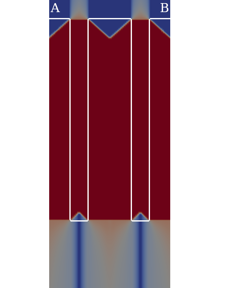
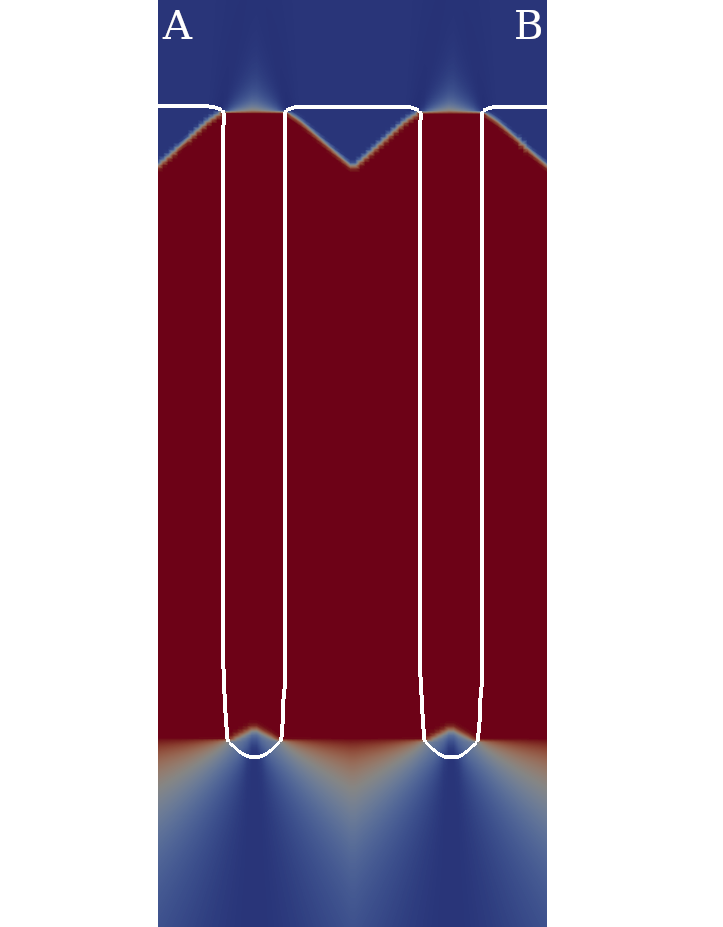
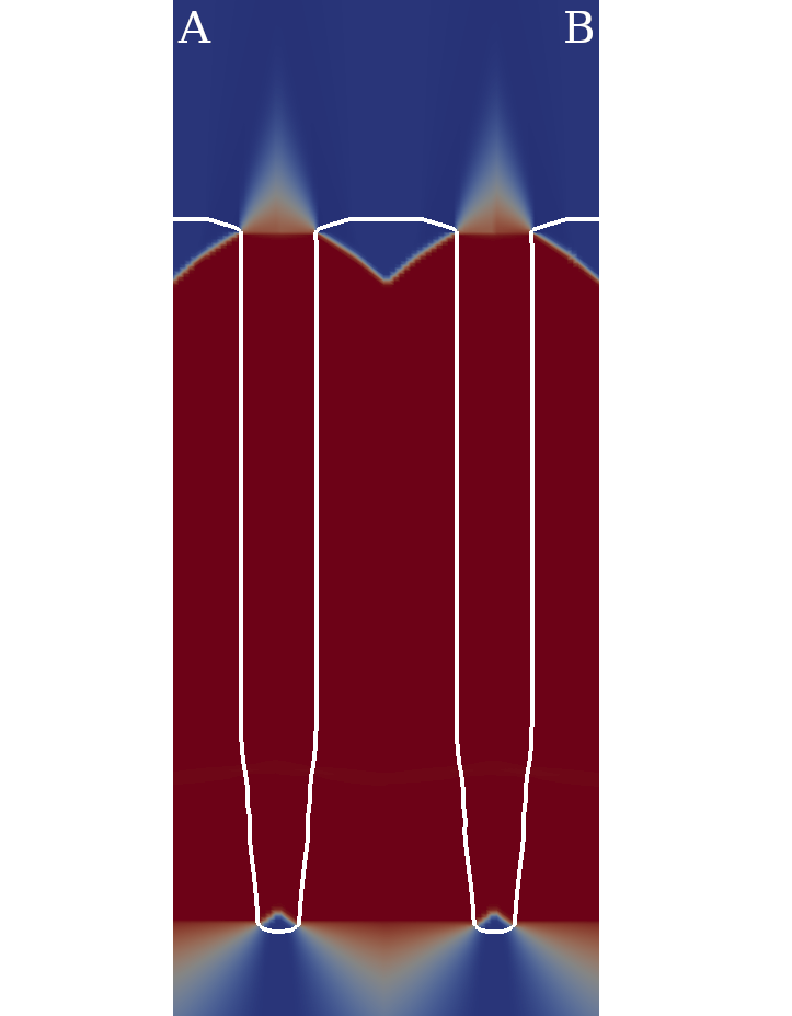
In Figure 5.8 a slice of the extended velocity field is shown for three different representative time steps during the simulation. The interface (surface of the structure) is shown by the white curve. The extended velocity is constant along the normals on the interface. The blue colors indicate a high etch rate, whereas red colors indicate a low etch rate (nearly zero). The high etch rates are mostly present in interface regions of the structure which face the top of the simulation domain which is the source of the ions. The IBE is highly anisotropic, thus at the corners of the MTJ pillars, the interface velocity abruptly changes, but are still well resolved. The rarefaction fans (continuous extension of the velocity field in concave areas of the interface) and the shocks (discontinuous extension of the velocity field in convex areas of the interface) are clearly visible.

As a first step, the serial performance of the proposed algorithms and data structures is evaluated, followed by the evaluation of the parallel performance.

Serial Performance Evaluation

The compute system VSC3 is used for the evaluation of this simulation example. The first benchmark compares (cf. Table 5.3) the serial run-time of the algorithms for both resolutions. The other metric shown in the table is the ratio of how often at least a single upwind neighbor is in the state Unknown compared to the total number of executions to the update algorithm (Un. up). This metric is a measure for optimal traversal. A traversal of all grid points is optimal, if each grid point is visited exactly once, yielding a ratio of zero. A ratio of 0.5 corresponds to visiting every grid point twice.

Table 5.3: Serial run-time (Run-Time) in seconds and the ratio of how often Unknown upwind neighbors (Un. Up.) were encountered compared to the total updates. Bold numbers indicate the fastest run-time for each resolution. The reference Algorithm 2 strictly requires a Heap to be correct (compute consistently all grid points), thus no results are obtained for the other data structures.

(a) Low Resolution Case

	Algorithm 2		Algorithm 3		Algorithm 5
Data Structure	Run-Time	Un. up.	Run-Time	Un. up.	Run-Time	Un. up.
Heap	0.265	0.0	0.258	0.034	0.190	0.262
Stack			0.196	0.418	0.200	0.416
Queue			0.162	0.077	0.177	0.259

(b) High Resolution Case

	Algorithm 2		Algorithm 3		Algorithm 5
Data Structure	Run-Time	Un. Up.	Run-Time	Un. Up.	Run-Time	Un. Up.
Heap	19.99	0.0	19.14	0.076	13.27	0.241
Stack			13.27	0.414	12.83	0.412
Queue			10.27	0.052	11.67	0.221

Algorithm 2 achieves the optimum (the dependencies to compute the velocity are always fulfilled). However, a disadvantage of the metric is that it neglects effects on the performance caused by access times and cache misses, thus the run-times do not correlate with the optimal traversal metric. Comparing the run-time for Algorithm 3 using a Heap and Queue data structure shows that although they have a similar ratio of Unknown upwind neighbors their run-times are vastly different. This shows the superiority of the less complex insert and getFirst operations of the Queue compared to the Heap. The Stack has the highest ratio of Unknown upwind neighbors, because the Stack implements a depth-first traversal, which often selects grid points further away from the interface first.

The run-times of Algorithm 2 are at least 1.3 times slower compared to Algorithm 3 and Algorithm 5, if considering a Stack or Queue. The shortest run-time is achieved using Algorithm 3 using a Queue data structure, yielding a serial speedup of 1.6 and 2.0 for the low and high resolution case, respectively. The high resolution case takes about 64 times longer than the low resolution case, which is approximately the same factor as for the number of grid points those cases differ. Thus a linear dependence of the run-time relative to the number of grid points is shown.

The difference between Algorithm 3 and Algorithm 5, using the Stack, is a reversed order of the grid points in the Band due to the stacks depth first traversal. The run-time is barely affected, because the ratio of Unknown upwind neighbors is about the same. For the Heap switching to Algorithm 5 is beneficial for the run-time, as it reduces the heap size manifesting in insert and getFirst operations to require a smaller share in run-time. The run-time of the Queue suffers from switching to Algorithm 5 as the ratio of Unknown upwind neighbors increases by a factor of four. The data structure used for the WQ (Band) in Algorithm 5 is less important compared to Algorithm 3, as the size of the Band is small. In Algorithm 5 the Band starts with a single grid point, compared to Algorithm 3 the Band contains about halve the Close Points (the other halve is used on the other side of the interface).

Parallel Performance Evaluation

The parallelization is evaluated for Algorithm 5 on one node of VSC3 for up to 16 threads utilizing all available physical cores⁴. Thread-pinning was used to avoid thread migration. The data is averaged over 10 iterations.

Figure 5.9 shows the run-time and parallel speedup of Algorithm 5. The shortest run-times are obtained for eight and 16 threads for the low resolution case and high resolution case, respectively. In both cases the Queue performed best, due to its serial superiority. Starting from two threads the serial-superior algorithm Algorithm 3 using a Queue is outperformed by the parallel algorithm regardless of the used data structure.

The highest parallel speedup (not lowest run-time) is achieved using the Heap, because using more threads further decreases the WQ size. Small WQ sizes are essential for the Heap as the insertion scales with the WQ size (Stack and Queue do not have this drawback).

The parallel speedup for the low resolution case using eight threads is 4.6 for the heap and the queue and 4.9 for the stack. For eight threads, the high resolution case has a parallel speedup of 4.5 for the stack, 5.3 for the queue, and 5.4 for the heap.

Using more than eight threads, requires the threads to be distributed over two memory domains (NUMA effects), leading to an increased run-time for the low resolution case (parallel speedup of 4.0) and only marginal speedup for the high resolution case (parallel speedup of 5.9) for all data structures. The memory is solely allocated by the first thread which resides on core 0 (part of the first processor), thus every thread running on the second processor has to indirectly access the memory. Additionally, threads running on different processors do not have shared caches further limiting speedup.

In Figure 5.10 the ratio of redundant computations and the ratio of Unknown upwind neighbors are shown. The ratio of redundant computations is investigated because Algorithm 5 does not use explicit synchronization between threads. Consequently, there might be cases where a grid point is computed more than once. As already mentioned in Section 5.5, the involved threads compute the same values. Considering two threads the ratio of redundant computations is below 0.01 %. For an increasing number of threads the ratio of redundant computations saturates, i.e., in the low resolution case below 1 % and high resolution case below 0.1 %. The ratio in the low resolution case is higher than in the high resolution case, as the number of grid points computed by a thread compared to the grid points where threads might interfere grow with different rates. A similar situation is found for the ratio between the volume and the surface of a sphere (square-cube law).

The ratio of Unknown upwind neighbors shown in Figure 5.10b declines slowly for increasing number of threads. That is because, if more threads are available, one of them might compute the Unknown upwind neighbors beforehand. The Queue has in the high resolution case a lower rate than the Heap, because the WQ has a better spatial locality.

Directly comparing the run-time of the serial execution of the FMM (Algorithm 2) to the best parallel execution of Algorithm 5 using the Queue shows that the run-time is reduced from 0.265 s to 0.038 s. The run-time reduction is attributed to a serial speedup of 1.5 and a parallel speedup of 5.6 for eight threads in the low resolution case. The high resolution case shows a reduction of the run-time from 19.99 s to 1.975 s utilizing all 16 threads. The serial speedup’s contribution is a factor of 1.7 and the parallel speedup’s contribution is a factor of 10.1.

In conclusion, for serial execution Algorithm 3 is the best choice and for parallel execution Algorithm 5 is the best choice. In both cases the Queue is superior to the other evaluated data structures, thus for the next benchmark example only the Queue is considered.

⁴ Evaluations considering simultaneous multithreading showed no noticeable speedup and have thus been excluded from presentation.

5.7.2 Thermal Oxidation

The results presented in this section were published in [56]. The developed velocity extension algorithm optimized for the full hierarchical grid (cf. Algorithm 7) is evaluated using the thermal oxidation example discussed in Section 1.1. The process model for the oxidation step consists of two physical problems [15]: (1) The transport and reaction of the oxygen (diffusion); and (2) the volume expansion due to the chemical conversion, silicon to silicon dioxide, which is accompanied by the material flow (displacement) of all materials above the reactive material (reaction). Each of the physical problems yields a velocity field at the interface. A particular challenge in this case is that one scalar and one vector velocity field has to be considered. This scenario requires two separate velocity extensions and specialized advection schemes for each extended velocity field.

The first physical problem (oxidant diffusing through the oxide), is mathematically described by the Poisson equation

$\begin{aligned} (5.11) & \frac{\partial}{\partial x_{i}} (D \frac{\partial C}{\partial x_{i}}) & = 0, \\ (5.12) & {- D \frac{\partial C}{\partial \vec{n}} |}_{Si/SiO_{2}} & = k C, {- D \frac{\partial C}{\partial \vec{n}} |}_{SiO_{2} /Si} = h (C_{0} - C), \end{aligned}$ with $C$ the oxidant concentration, $D$ the diffusion coefficient, $k$ the reaction rate, $h$ the gas-phase mass-transfer coefficient, $C_{0}$ the equilibrium concentration in the oxide, and $\vec{n}$ the normal to the corresponding material interface. This gives a reaction rate at the silicon interface which is ultimately transformed to a scalar velocity field $v$ at the Cross Points of the gas interface (surface of the structure).

The second physical problem (volume expansion from the chemical reaction and displacement of materials) is mathematically described by a creeping flow

$\begin{matrix} (5.13) & \frac{\partial S_{i j}}{\partial x_{i}} = 0, \end{matrix}$

with $S_{i j} = - p \cdot δ_{i j} + σ_{i j}$ denoting the Cauchy stress tensor, $p$ the pressure, and $δ_{i j}$ the Kronecker delta. The shear tensor $σ_{i j}$ uses the Maxwell visco-elastic fluid model which, combined with further simplifications, yields the system of Stokes equations

$\begin{array}{r} (5.14) & μ Δ \vec{v} = \nabla p, \\ (5.15) & \nabla \cdot \vec{v} = 0, \end{array}$ with $\vec{v}$ the vector velocity field and $μ$ the dynamic viscosity. The vector velocity field $\vec{v}$ is the second velocity field which needs an extension for this simulation.

Simulation Parameters

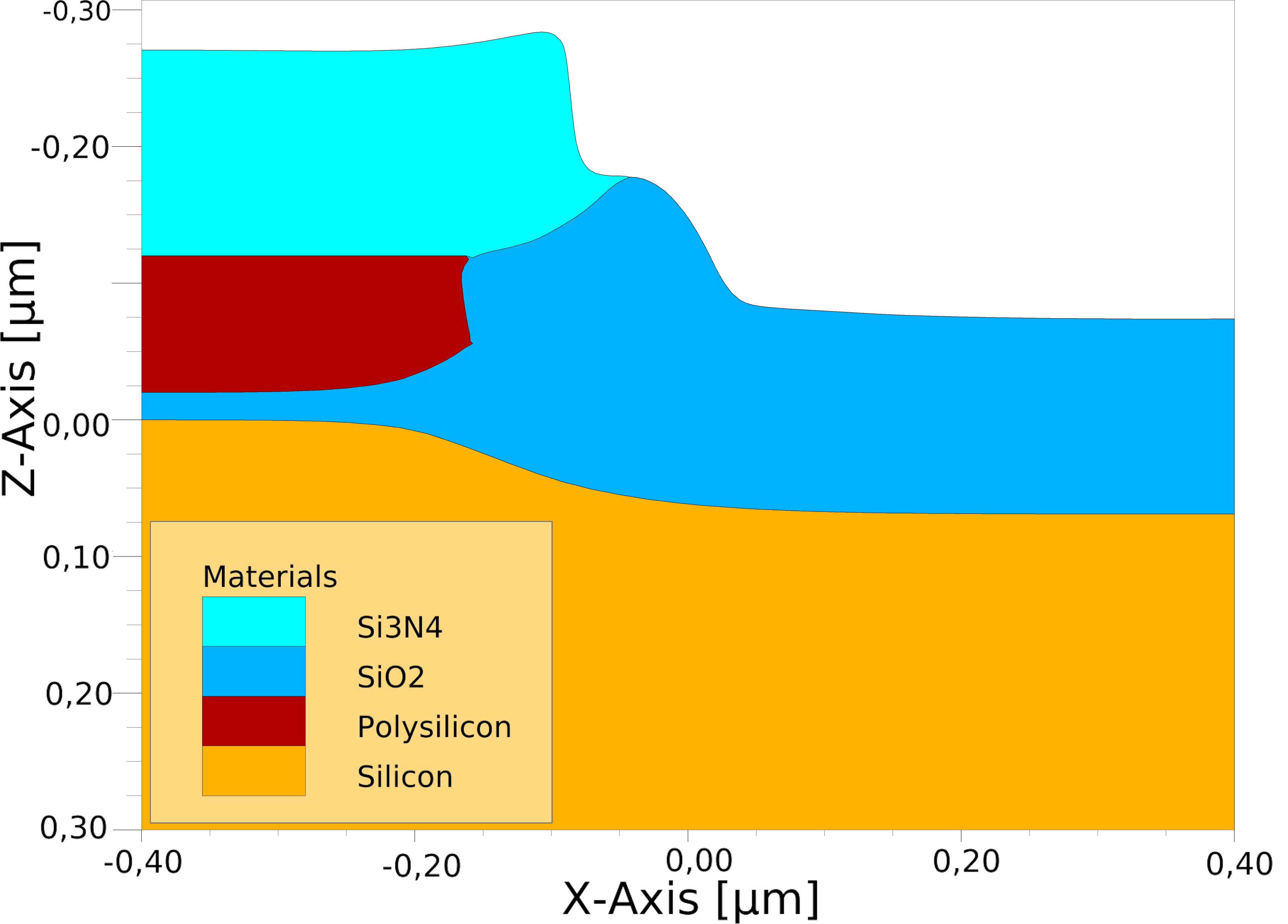
The simulation is performed on a rectilinear simulation domain with symmetric boundary conditions, representing a unit domain of the full wafer. The simulation domain covers a volume of 1.6 µm $\times$ 0.8 µm $\times$ 1.0 µm. The material stack consists from bottom to top of: 0.3 µm bulk silicon, 0.02 µm padding silicon dioxide, 0.1 µm buffer polysilicon, and 0.15 µm hard mask silicon nitride. Figure 5.11 shows the detailed topography before the thermal oxidation step and a slice of the aftermath of the 15 min thermal oxidation step at a temperature of 1000 °C. The bird’s beak formed by the silicon oxide between the silicon and the polysilicon is well resolved.

The single block covering Level 0 contains $40 \times 80 \times 40 \hat{=} 128 000$ grid points. The data of the hierarchical grid on Level 1 is shown in Table 5.4. During the simulation which requires a total of 27 time steps, every third time step the hierarchical grid is re-gridded to fit the current topography of the structure. The number of blocks varies between 17 and 34, with the general trend that the number goes up due to an increased complexity of the material regions. The number of blocks is important for the parallelization, because the unmodified algorithm Algorithm 7 (using red parts) and the corresponding Algorithm 8 (not using advances highlighted in blue) are directly limited by the number of blocks.

Table 5.4: Evolution of the number of blocks and total number of grid points on Level 1 of the hierarchical grid shown for all time steps.


Time Step	Number of Blocks	Number of Grid Points


0	18	$536 704$
3	22	$492 544$
6	18	$503 808$
9	20	$620 544$
12	17	$566 592$
15	28	$683 840$
18	18	$774 016$
21	30	$764 992$
24	33	$868 928$
27	34	$969 536$

The number of grid points on Level 1 varies (between $492 544$ at the beginning and $969 536$ grid points at the end of the simulation). There is no direct correlation between the number of blocks and number of grid points. The general trend for more grid points during the simulation, caused by the increased complexity of the material regions, also holds for the number of grid points.

Performance Evaluation

In Figure 5.12 the run-time and parallel speedup are shown for the velocity extension. The run-times were obtained using the ICS compute system utilizing up to 10 cores. The run-times labeled new are based on using the new Algorithm 7 with all its changes once for the scalar velocity case and once for the vector velocity case.

The run-times labeled Original are obtained from previous versions of the velocity extension. For scalar and vector velocity cases different different algorithms are used as base line. In particular Original Vector Velocity Extension uses the original FMM (Algorithm 2). It employs a single global priority queue (implemented via a heap) for all blocks on a level of the hierarchical grid. This does not allow for any parallelization. The minor variations in the run-time for different number of threads is created by noise, e.g., originating from the operating system.

The Original ScalarVelocity Extension uses Algorithm 7 without the proposed changes and optimization for the hierarchical grid presented in Section 5.6. Thus, the global Heap is replaced by the Queue on a per block basis. The proposed algorithm has 4 % slower serial run-time, because the performance is impacted by the modified exchange step and for a single-threaded execution global synchronization barriers are irrelevant.

The parallel speedup for the scalar velocity extension maxes out at 6.6 for 10 threads. Comparing this to the original implementation which only reached a parallel speedup of 4.1, shows an improvement of 60 %. The parallel speedup of the original implementation starts to saturate at four threads, because the implicit load-balancing from the utilized thread pool deteriorates. The deterioration is caused by the limited number of tasks which is directly related to the number of blocks on a level, e.g., 17 blocks and 10 threads mean that three threads will get only a single block to process thus balancing the different workloads per block is not possible.

The new vector velocity extension reaches a parallel speedup of 7.1 for 10 threads. This is an improvement compared to the scalar case, which is caused by the three times higher computational load at each grid point, because the vector velocity has three components in a 3D simulation. The serial run-times for the scalar and vector velocity extension differ only by 43 % instead of the 200 % (each component of the vector adds 100 % run-time) expected from a three times as high workload per grid point. This indicates that most of the run-time is spent on checks and ordering of the grid points (memory intensive) rather than velocity computations. A further extension of the proposed algorithms is to extend the scalar and vector velocity together, if the process model allows it.

5.8 Summary

In this chapter the computational step Velocity Extension has been discussed in detail. First the extension from the Cross Points to the Close Points, which is trivially parallelizable, was presented. Then the original FMM used for the velocity extension was presented, because it is the basis and reference for the developed algorithmic advancements. The key challenge in parallelizing the FMM for the velocity extension was to overcome the use of a heap data structure to determine the order in which the velocity is extended to the grid points of a block.

Based on an interpretation of the FMM through graph theory a new approach was developed where different data structures were employable to determine the order of the extension. The algorithmic changes were evaluated on a Cartesian grid using a single thread, where a serial speedup ranging from 1.6 to 2.0 for the velocity extension was measured. In particular, three different data structures Heap, Stack, and Queue were evaluated: The Queue performed best.

The changes to the data structure enabled a parallelization of the algorithm on a Cartesian grid. The parallelization was performed without any explicit synchronization constructs, thus redundant computations (points are computed multiple times) manifested. However, redundant computations count less than 1 % for 16 threads. Depending on the spatial resolution parallel speedups ranging from 4.9 to 5.3 using eight threads were achieved. Overall, a parallel speedup of 5.9 for 16 threads was achieved, further improvements being limited by NUMA effects.

Finally the proposed algorithm was adapted to a hierarchical grid, by reducing global synchronization barriers present in the original algorithm. The global synchronization barriers were reduced by developing a specialized exchange mechanism between blocks, which does not require additional synchronization barriers. This allowed for a parallel speedup of 7.1 for 10 threads, which is 60 % higher compared to the original algorithm. A direct comparison between the extension of a scalar and a vector velocity field showed that most of the run-time is spent on the checks and ordering and not on the computation of velocities.