Chapter 6 Load-Balanced Parallel Re-Distancing

This chapter presents the details of the computational step Re-Distancing and the developed load-balanced parallel FMM approach. Re-Distancing restores the signed-distance property of the level-set function without altering the interface position. Aside from discussing other approaches, the focus is on introducing the new block decomposition for the FMM which allows for superior parallel efficiency compared to previous approaches.

In principle, there are three strategies to compute the signed-distance function relative to a given level-set function:

• • Re-initialization, uses the level-set equation with a velocity field, which converges to a signed-distance function.

• • Direct computation of the signed-distance, which is based on finding the closest point on the interface.

• • Eikonal equation, considers the computation of the signed-distance as a special case of the more general Eikonal equation.

The first two approaches are briefly discussed below, however, the focus is on solving the Eikonal equation (see Section 6.1), because the FMM for which the block decomposition was developed belongs to the class of Eikonal equation solvers.

Previous shared-memory parallelized approaches using the FMM suffer from load-imbalances, if the ratio of blocks (on a level of a hierarchical grid) per thread is low, e.g., below 10 [62]. Therefore, the core contribution presented in this chapter and published in [159], is a block decomposition approach to enable load-balancing. The developed block decomposition approach temporarily increases the number of blocks on all levels of a hierarchical grid (Section 6.2).

In the last section, the developed block decomposition approach is evaluated via a parameter study on the granularity of the decomposition and frequency of the data exchange steps between blocks (Section 6.3). For the evaluation a generic test case (a point source) for Eikonal solvers (Section 6.3.1) is considered, as well as, two representative example interfaces stemming from process TCAD simulations (Section 6.3.2 and Section 6.3.3).

The discussion continues with an overview of the strategies to compute the signed-distance.

Re-initialization

Re-initialization strategies use the level-set equation itself, employing a specific velocity function which ultimately leads to

\begin{align} \frac {\partial \Phi }{\partial t} & =\text {sgn}\left (\Phi ^0\right )\left (1-|\nabla \Phi |\right ),\label {eq:steadystate} \\ \Phi \left (\vec {x},0\right ) & =\Phi ^0\left (\vec {x}\right ), \end{align} where \(\Phi ^0\) is the given distorted level-set function and \(\Phi \) is the desired signed-distance function. The \(\text {sgn}\) term forces that the sign of the level-set function does not change during the re-initialization, i.e., inside stays inside and outside stays outside.

Equation (6.1) is solved numerically to a steady state (advanced for some time steps until the difference between two consecutive solutions \(\Phi \) is below a threshold), yielding the signed-distance function \(\Phi \) [160]. The signed-distance property of \(\Phi \) follows directly from (6.1) by using \(\frac {\partial \Phi }{\partial t}=0\) (due to the steady sate) and moving \(|\nabla \Phi |\) to the left hand side (compare (4.25)).

The drawback of this approach is that the interface is typically moved during the process; this leads to smoothening of sharp features, e.g., corners, and is obviously counterproductive in a process TCAD simulation setting as critical device features would deteriorate. The movement of the interface is dependent on the number of iterations necessary to reach the steady state, where a higher number of iterations results in a bigger deviation of the interface position. The number of required iterations increase the further the initial \(\Phi ^0\) deviates from a signed-distance function.

Improvements to this method were made by modifying the used velocity [161, 162, 163]. These advancements yield the same steady state solution, but allow for a faster convergence to the steady state, as well as a smaller disturbance of the interface position.

Direct Computation of the Signed-Distance

The methods belonging to this strategy compute the signed-distance by calculating the closest point on the interface, i.e., minimizing the distance to the interface. The methods are similar to a gradient descent algorithm [164]. The closest interface point is computed by first using the gradient and the level-set value for an educated guess of the interface location. The quality of the educated guess is high, if the given level-set function is close to a signed-distance function.

The educated guess is then refined by directional optimization [165]. Conceptually similar methods based on the Hopf-Lax formula are presented in [166, 167].

Direct computation of the distance methods are easy parallelizable, because the computations on different grid points are independent [168]. The main disadvantage, however, is that the level-set function has to be close to a signed-distance function for optimal efficiency. Achieving high accuracy at corners is challenging, because the interface normals are ill-defined at those locations. The accuracy of methods belonging to this class is bound by the interpolation scheme used by the directional optimization to determine the exact interface position.

6.1 Eikonal Equation

The Eikonal equation is developed to describe a wave front emerging from \(\Gamma \) and marching through \(\Omega \)

\begin{align} \left |\nabla \Phi \left (\vec {x}\right )\right | & =F\left (\vec {x}\right ),\quad \vec {x}\in \Omega , \\\Phi \left (\vec {x}\right ) & =G\left (\vec {x}\right ), \quad \vec {x}\in \Gamma , \end{align} with the given wave speed \(\frac {1}{F\left (\vec {x}\right )}\) and departure time \(G\). Using a wave speed of one and a zero departure time the distance to the interface is computed.

The Eikonal equation has applications in various areas of science and engineering, such as seismic processing [169, 170, 171], path-finding [172, 173, 146], and 3D imaging [106]. Therefore, there are several available computational approaches to solve the Eikonal equation. A short overview of the approaches to solve the Eikonal equation on Cartesian grids is given in [146]¹. The most widely-used solution approaches are (further details provided in the following):

• • Fast sweeping method (FSM)

• • Fast iterative method (FIM)

• • FMM

The methods use a set of seed points (representing the discretized interface \(\Gamma \) on the grid). For Re-Distancing those seed points are the same as the Close Points (cf. Section 5.2). It is possible to also re-compute the signed-distance on the Close Points increasing the accuracy of the solution, but doing so alters the interface position [162]. The change of the interface position is strictly unwanted (see previous reasoning concerning the preservation of the process TCAD critical geometrical features of the to-be-simulated devices), thus Close Points are never modified.

All methods to solve the Eikonal equation have an Update algorithm (cf. Algorithm 9) in common, which solves the discretized Eikonal equation

\begin{align} \begin{bmatrix} \max \left (D_{ijk}^{-x}\Phi ,D_{ijk}^{+x}\Phi ,0\right )^2+ \\ \max \left (D_{ijk}^{-y}\Phi ,D_{ijk}^{+y}\Phi ,0\right )^2+ \\ \max \left (D_{ijk}^{-z}\Phi ,D_{ijk}^{+z}\Phi ,0\right )^2\phantom {+} \end {bmatrix}^{\frac {1}{2}}=F_{ijk}, \label {eq:upwind} \end{align} with \(D_{ijk}^{+x}\Phi \) the forward difference approximation and \(D_{ijk}^{-x}\Phi \) the backward difference approximation to the spatial derivative \(\frac {\partial \Phi }{\partial x}\). The discretization by (6.5) is establishing an upwind scheme, because it uses in each spatial dimension only grid points with lower \(\Phi \) values (Algorithm 9 Line: 5). The forward and backward differences are typically computed using a first-order scheme (cf. Section 2.1), which requires a stencil containing direct neighboring grid points (grid points for which the sum over all spatial dimensions of the absolute index differences is equal to one).

Higher order schemes require a wider stencil (containing more grid points), a second-order scheme for example is presented in [177]. The higher order schemes are out of scope for process TCAD simulations: In case the interface is not smooth, e.g., at interface corners, the higher order of those schemes is reduced. In order to solve (6.5) using the first-order scheme for \(\Phi _{ijk}\), rearranging the terms of (6.5) reveals the structure of a quadratic equation in \(\Phi _{ijk}\)

\begin{align} \underbrace {\sum _{i\in \{x,y,z\}}\Delta _i^2}_{=\,a} \Phi _{ijk}^2+\underbrace {-2\sum _{i\in \{x,y,z\}}\Delta _i^2T_i^2}_{=\,b}\Phi _{ijk}+\underbrace { \sum _{i\in \{x,y,z\}}\Delta _i^2T_i^2-F_{ijk}}_{=\,c}=0, \end{align} with \(T_i\) the \(\Phi \) value of the chosen upwind neighbor in the corresponding spatial dimension. This equation is solved in Algorithm 9 Line: 14. In case no real solution exists (the quadratic has two complex roots) the largest upwind neighbor is removed (its contributions are set to zero cf. Algorithm 9 Lines: 17-19). Then the procedure to solve the quadratic equation is restarted. If only a single dimension has nonzero contributions, a real solution to the quadratic is guaranteed to exist.

FSM

The FSM [178], computes the solution by repetitively sweeping the computational domain. A sweep computes for every grid point an Update by considering only neighbors in, e.g., negative x/y/z-direction. For the next sweep the directions are changed considering the previous example: positive x-direction and negative y/z-direction. A full sweep consist of all the \(2^d\) (\(d\) is the number of dimensions) possible combinations of sweep directions. Improvements to the FSM that lock some of the grid points, i.e., locked sweeping method (LSM) such that not all grid points have to be computed in a sweep, are presented in [179]. The FSM terminates, if the difference of the solution between two consecutive full sweeps is below a threshold. The threshold is selected based on the desired accuracy of the solution. In case of a constant speed function \(F\) the solution is already reached after a single full sweep, thus \(2^d\) sweeps are necessary for Re-Distancing.

The Eikonal equation is a minimization problem, therefore, the solution is given by the smallest computed value at each grid point over all sweeps of a full sweep. Therefore, the individual sweeps may be computed in parallel allowing up to \(2^d\) threads simultaneously. If more threads are available, a sweep is additionally parallelizable because all grid points with the same sum of their indices are independently computable (a strict order applies to the order of the sum of the indices) [180, 181].

FIM

The FIM [182, 183] (as its name suggest) iteratively uses the Update function on all grid points. The FIM terminates when the difference of the solution between two iterations falls below a threshold value. The threshold corresponds to the desired accuracy of the solution. In comparison with the FSM the FIM considers always all neighbors. Improvements to the FIM are that for an iteration only selected grid points are computed again [184]. For a constant speed function \(F\) the iteration terminates in a maximum number of iterations, which is equivalent to the diameter of the domain in grid points. Parallelization for the FIM is straightforward, because the update for all grid points is performed independently in each iteration [185, 186, 187].

FMM

The FMM as portrayed previously in Section 5.3 is unique in the sense that it is a single pass algorithm (every grid point is computed only once). The modifications presented in Chapter 5 for parallelizing the FMM are not applicable to the FMM used in Re-Distancing, because the dependencies (upwind neighbors) of the grid points are not known beforehand.

Thus the approaches for parallelizing the FMM for Re-Distancing (or more generally the Eikonal equation) are based on domain decomposition. The domain is decomposed and an instance of the FMM is performed independently on each sub-domain. Consequently, this requires a merging of the solution from the different sub-domains. The merging inevitably leads to iterative rollback mechanisms for any domain decomposition approach. The role back mechanism invalidates the solution on parts of the domain and initiates a re-computation of the solution, thus the single pass property of the FMM is lost [188]. There are several approaches trying to limit the number grid points affected by rollbacks [189, 190]. The approaches differ by whether the sub-domains are overlapping, considered neighbors of the sub-domains, and exchange frequency between the sub-domains.

The exchange frequency between sub-domains is controlled by a parameter called stride width which limits how far the solution may advance before a mandatory data exchange takes place [61, 171]. So far the effect on the performance of the stride width has not been studied for hierarchical grids. Choosing a small stride width reduces the by the rollbacks affected points, whilst a large value reduces the number of synchronization barriers due to the reduced data exchanges.

An overview of available FMM approaches in a single block and multi-block context is summarized in Figure 6.1.

In what follows, we consider the block decomposition to only apply to the Re-Distancing and not interfere with the given hierarchical grid itself, which is tailored to solution requirements of the physical simulation steps, i.e., optimal grid resolution in areas of interest, such as corners, to optimize robustness, accuracy, and computational complexity.

6.2 Block Decomposition

Previous analyses show that, if the number of blocks is about 10 times bigger than the number of threads, the load-balancing is possible [62], increasing parallel efficiency. To artificially increase the number of blocks on a level of a given hierarchical grid, a decomposition of the available blocks into sub-blocks is necessary. Sub-blocks are exactly like blocks, but to differentiate from the original blocks the distinguishable descriptor, sub-blocks, is used.

The naive decomposition approach splits the largest block into two sub-blocks along its longest side until the desired number of blocks is reached. This is not a viable option because this approach is inherently serial due to the selection of the largest block. Additionally, there is no lower bound on the block size, so excess creation of tiny sub-blocks, e.g., one grid point wide blocks, will deteriorate performance (as those blocks would still need a ghost layer, which would be bigger than the actual block).

In contrast, a superior approach is developed and presented in the following. The approach decomposes blocks only, if they are larger than a given block size into sub-blocks smaller or equal in size of the block size (Figure 6.2). For a chosen block size of 10, only the larger block (\(14\times 13\)) is split, whilst the smaller block (\(7\times 5\)) remains unchanged. The larger block is simultaneously split into four sub-blocks, two with a size of (\(7\times 7\)) and two with a size of (\(7\times 6\)). This approach favors parallelism, because every block is split independently. Additionally, the block size parameter allows to take cache sizes of the underlying hardware into account, because the block size parameter gives tight control over the created sub-block sizes. The sub-block size has direct influence on the required memory.

To deploy the decomposition onto a hierarchical grid the neighbor relations between the (sub-)blocks have to be computed and the ghost layers have to be checked for overlaps, identifying grid points which require a synchronized exchange. During the preparation the blocks are split into sub-blocks, based on the proposed block size. Finally, the multi-block FMM is applied [62]. In summary, the developed advancements of the parallel FMM consist of three sub-steps: Block decomposition, sub-block allocation, and ghost layer computation. Figure 6.3 illustrates the algorithm via a flow chart and each step is discussed in the following.

Block Decomposition

The decomposition of a block is independent from the decomposition of other blocks, thus decomposing the blocks is inherently parallel. Additionally, the decomposition is also independently applicable to all spatial dimensions, therefore, it is sufficient to present the one-dimensional case. For a given block by its start index \(S\)², its original size \(N\) in grid points, and the chosen block size \(B\), the number of sub-blocks \(M\) is computed by

\begin{equation} M=\left \lfloor \frac {N+B-1}{B}\right \rfloor . \end{equation}

Thus there are \(M\) sub-blocks necessary so that none of them has to be bigger than \(B\). The individual starting index \(S_i\) of the sub-blocks and the size \(N_i\) for the sub-block \(i\) are computed using

\begin{equation} N = M \cdot q+r, \end{equation}

with \(q\) the unique quotient and \(r\) the remainder. So, \(S_i\) and \(N_i\) are given by

\begin{align} S_i & =\begin{cases} S+i(q+1) & \text {for } i<r \\ S+(i-r)q+r(q+1) & \text {for } i \ge r \end {cases}, \\ N_i & =\begin{cases} q+1 & \text {for } i<r \\ q & \text {for } i \ge r \end {cases}. \end{align} The created sub-blocks vary in size by at most a single grid point, because of their definition. The case occurs, if \(N\) is not divisible by \(M\). Figure 6.4 shows an exemplary block decomposition, with all variables graphically shown.

Consider an alternative approach where the original block is cut into \(B\) sized sub-blocks except for the last sub-block which is only \(r\) grid points wide. This alternative approach is inferior to the proposed approach because in case the last sub-block with size \(r\) is only one grid point wide requires frequent data exchange steps which deteriorate the parallel performance or in case of infrequent data exchanges the rollbacks affect many points.

In the higher dimensional case, the block size is equal in all spatial dimensions for the standard case where the grid resolution (distance between two grid points) is the same. If the grid resolution is different along spatial dimensions, different block sizes along the different spatial dimensions are appropriate. If the sub-blocks are most similar to a cube, the spatial locality of the blocks is increased. This is not further investigated in this thesis, but might offer an interesting path for future research, especially for high aspect ratios of the grid resolution along different spatial dimensions.

(Sub-)Block Allocation

After the sub-blocks are defined, memory for the grid points, ghost layer and, the FMM’s binary heap has to be allocated (cf. Figure 6.3). The heap is preallocated to avoid costly re-allocations during the execution of the FMM in case the heap outgrows the initial chosen size. The preallocation size is chosen such that all grid points of a block are able to fit, thus no re-allocations are necessary. The preallocation allows to use an indexed lookup into the heap, if grid points are already present, shortening the time required to update the priority (key) for a grid point.

Blocks which have not been decomposed require only the allocation of the heap data structure. The whole process is parallelized over the sub-blocks, enabling the parallel execution of up to the number of sub-blocks threads. If less threads are available load-balancing takes place, because sub-blocks which do not require a decomposition take significantly less time. A synchronization barrier is needed to proceed to the next step.

Importantly, no data is copied during the block allocation to the sub-blocks. Data is only copied directly before and after the FMM is executed. This enables an efficient reuse of the sub-blocks over several time steps of a full process TCAD simulation, as long as the underlying hierarchical grid does not change.

Ghost Layer Computation

The neighboring sub-blocks (in the following, referred to as neighbors) are computed in two steps: 1) Neighbors from the same original block and 2) neighbors from a different original block (cf. Figure 6.3). The neighbors from the same original block are computed by index calculation, because the original block is regularly decomposed. Those neighbors either share a full face (i.e., all grid points of one of the axis-aligned sides) or no grid point at all. The neighbors from a different original block, are computed with a pairwise overlap computation of their ghost layer, for the sub-blocks. In the overlap computation only sub-blocks which originate from a neighboring blocks of their original block are considered. Thus the performance is increased, because not all sub-blocks have to be considered. The grid points in the ghost layer are marked to belong to the externally set grid points³ or to the to-be-synchronized grid points, i.e., they are covered by a neighboring sub-block. In the latter case, the grid points are collected on a per block basis to allow for an efficient data exchange with the neighboring sub-blocks. The parallelization strategy is the same as the one employed for the sub-block allocation, allowing high parallelization.

6.3 Benchmark Examples and Analyses

The proposed block-based FMM is evaluated based on three benchmark examples. The first example is a Point Source example. The other two (Mandrel and Quad-Hole) examples are inspired by process TCAD simulations.

The results are obtained from the benchmark system VSC4 (cf. Section 3.2). Different values for the parameter block size are compared as well as different values for the parameter stride width.

6.3.1 Point Source

The Point Source example is a fundamental test case for benchmarking Eikonal solvers [61, 146, 171]. The computational domain covers the cube \([-0.5,0.5]^3\) using a Cartesian grid (Level 0 of a hierarchical grid). The spatial discretization has 256 grid points along each spatial dimension yielding a total of \(16\,777\,216\) grid points. The domain boundary conditions are chosen to be symmetric in all spatial dimensions. At the center (\([0,0,0]\)) a single grid point is set to be the source point (interface). The speed function is constant, \(F=1\). Thus the iso-contours of \(\Phi \) are spheres centered on the source point (cf. Figure 6.5a).

First, the modified step Setup FMM (cf. Figure 6.3) is analyzed and then the performance of the FMM itself is analyzed.

Setup FMM

The measured run-times are shown in Figure 6.5b for block sizes ranging from 256 (a single block) down to eight (\(32\,768\) blocks). In case of block size 256 no decomposition is performed, giving no parallelization possibilities. In the other cases the block is decomposed, creating a significant serial overhead, due to memory allocation and additional ghost point computations. Parallel execution on the other had is now possible, yielding (depending on the chosen block size and used number of threads) a shorter run-time than the base case without decomposition. For block sizes of eight or 16 the break even point is never reached because the enormous number of blocks (\(4\,096\) and \(32\,768\), respectively), each with only a little computational, load suffer from synchronization overhead which materializes with more than four threads. Usage of computational resources from the second processor (more than 24 threads) did in no case increase the performance as NUMA effects add to the already memory-bound problem.

FMM

To analyze the run-time of the advanced FMM itself and the parallel speedup, Figure 6.6 shows the run-time and speedup for block sizes from eight to 256 and for different values of stride width measured in multiples of the grid resolution. In case no decomposition takes place (block size 256), the run-time is hardly affected by the used number of threads as well as from the stride width. The next finer block size 128, creates eight blocks. A serial speedup is measured for stride widths smaller than 20. The speedup ranges from 1.01 (stride width of 0.5) to 1.14 (stride width of 3.5), the cause of the speedup is the reduced number of grid points per block and smaller heap sizes and better cache efficiency due to data locality. The parallel speedup saturates for eight threads, because there are only eight blocks available. Small stride widths perform better, because the source point is located on a single sub-block, allowing computations on other sub-blocks only after the first exchange step, which is caused earlier by a smaller stride width.

For smaller block sizes a serial speedup is observed for stride widths of less than 10, reaching the highest serial speedup of 1.21 for a block size of 64 and a stride width of 3.5. If the used number of threads is high, large stride widths perform better, because the computational load per sub-block is decreasing rapidly, but the overhead caused by the synchronization decreases slower in comparison (following a square-cube-law). The peak parallel speedup of 19.1 using all 24 threads of a single processor is achieved with a block size of 32 and a stride width being equivalent to infinity (i.e., \(10\,000\)).

Utilizing the second processor only gives a speedup for block sizes of 64 and 32 and large stride widths, bigger than (depending on the block size) 10 and 50, respectively. The reason is that the typical computational load per task is to small too compensate the synchronization overhead. The same parameters of block size and stride width as for the usage of a single processor yield the peak parallel speedup of 20.7 for 48 threads: NUMA effects limit parallel performance, because frequent (especially for small stride width) synchronization steps cause a task rescheduling. The task rescheduling in OpenMP does not consider memory layout, resulting in many indirect memory accesses, because a block may have been processed earlier by a thread located on a different processor.

The next evaluation example is based on a process TCAD simulation and a hierarchical grid.

6.3.2 Mandrel

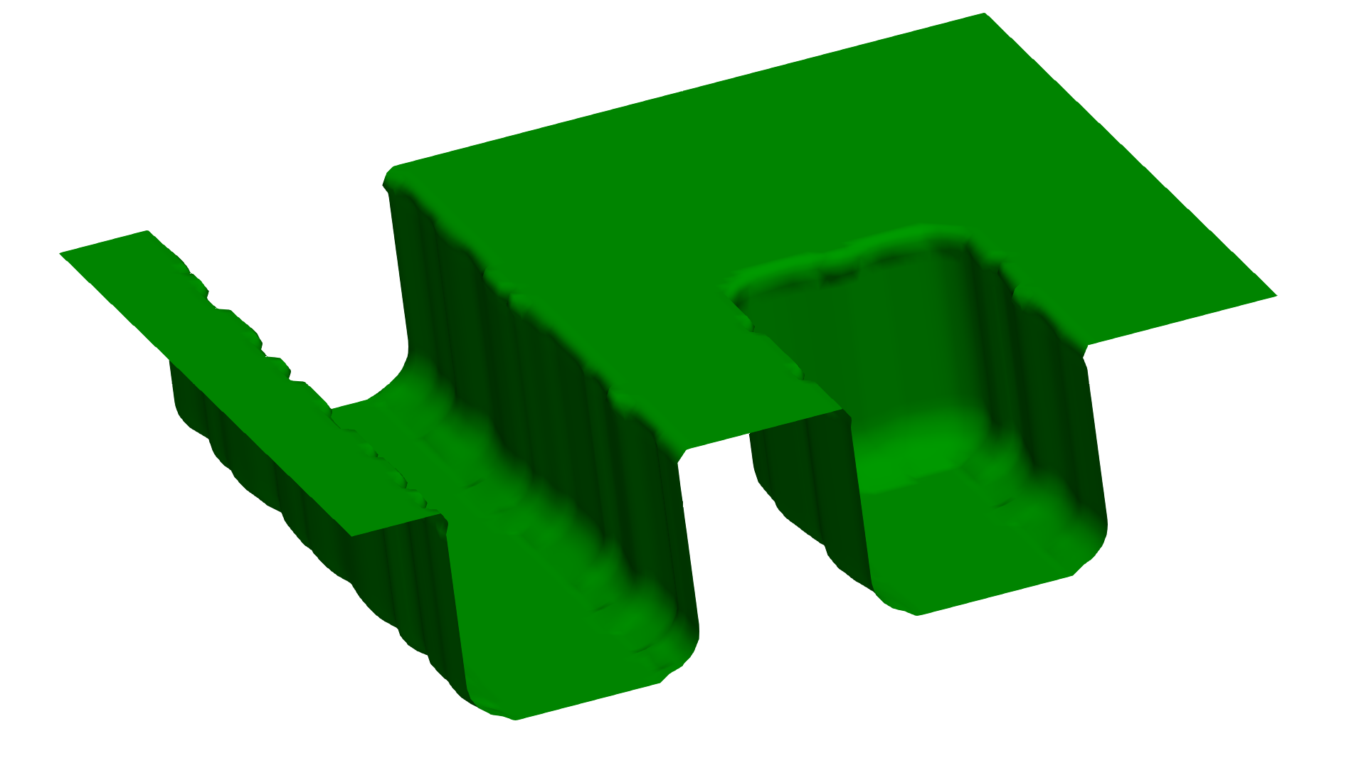
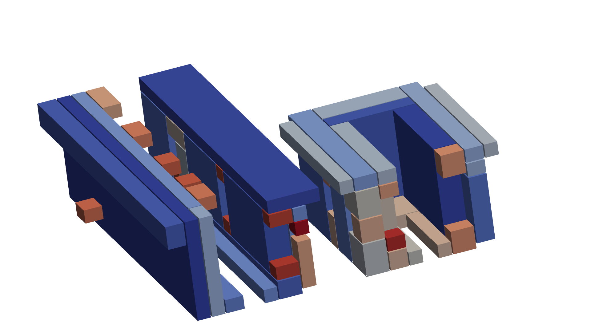
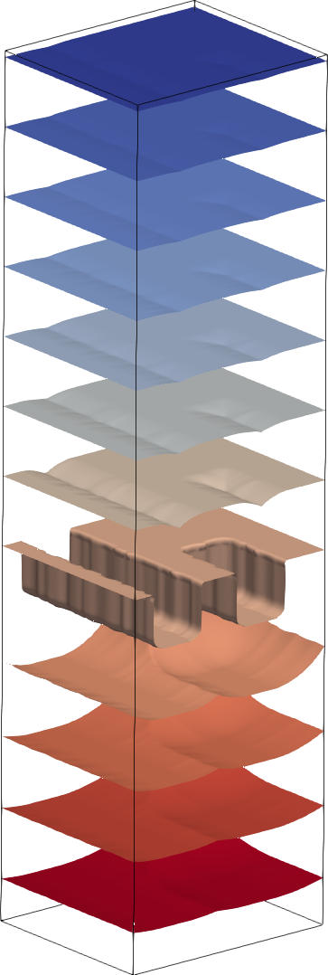
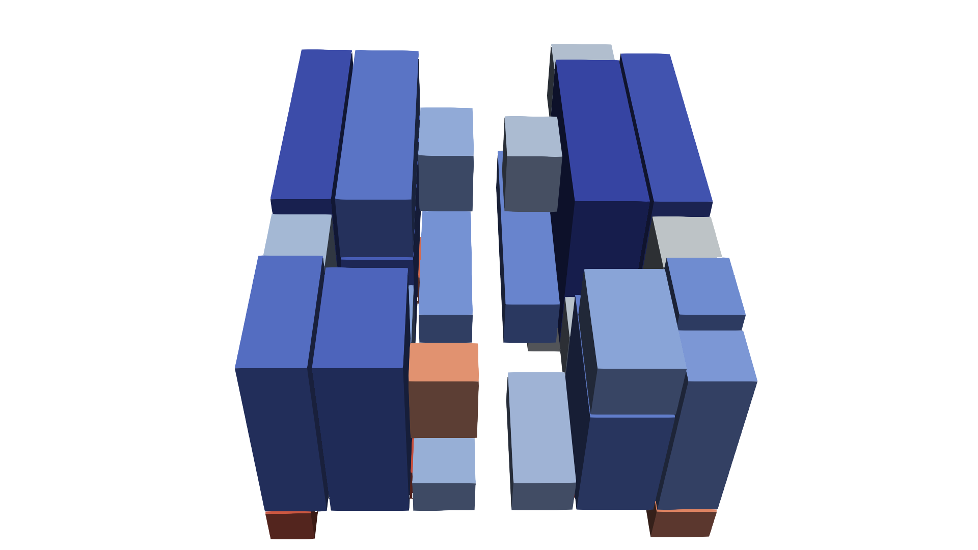
The Mandrel benchmark example is taken from a representative process TCAD simulation, where two trenches are etched into a silicon waver. One trench spans the full width of the simulation domain, and the other only half. Again, symmetric boundary conditions are used. Figure 6.7a shows the 0-level-set for which the signed-distance function is computed (constant speed function \(F=1\)). The hierarchical grid consists of two levels. The block on Level 0 has a size of \(84\times 72\times 312\), totaling about 1.8 million grid points. On Level 1 there are 78 blocks with their sizes ranging from \(12\times 12\times 12\) to \(12\times 288\times 84\), totaling about 2.5 million grid points. In Figure 6.7b the blocks on Level 1 are visualized: They are placed around the trenches. The signed-distance field (computed relative to the interface) is visualized via iso-contours, as shown in Figure 6.8a.

First, the Setup FMM is investigated and then the performance of the FMM itself is analyzed on both levels of the hierarchical grid separately.

Setup FMM

Figure 6.8b shows the measured run-time on VSC4. The setup time for the Mandrel example profits from using more threads, even without the block decomposition, because on Level 1 there are natively 78 blocks which may be processed in parallel. The shortest run-time is achieved using eight threads. Considering also the run-time with the block decomposition, a serial overhead materializes (due to memory allocation) with the added benefit of a better parallel scalability. The shortest run-time is achieved for a block size of 75 using 16 threads. Increasing the number of threads beyond 16 increases the run-time, especially for 48, threads when both processors are utilized. This is attributed to NUMA effects and the total lower computational load (maximum 2.5 million grid points) compared to the Point Source example (16 million grid points).

FMM Level 0

In Figure 6.9 the run-time and parallel speedup for the Level 0 of the Mandrel example are shown. A larger stride width performs better in the case where the block is not decomposed. Compared to the Point Source example where little influence of the stride width has been found: The run-time is an order of magnitude shorter and reveals that the introduced overhead by the restarts of a small stride width is not negligible.

Choosing a block size of 200 creates two sub-blocks (the domain is split along the z-axis). A serial speedup is not observed, because the split almost aligns with the interface, which already partitions the domain in two independent sets. The run-time is decreased for parallel execution only for a stride width from 10 to 50. For the maximum stride width of \(10\,000\) no parallel speedup is observed, because the interface and thus all initial points are located in a single sub-block, which forces a sequential computation of the sub-blocks. For stride widths smaller than 10 the restart overhead is too large to reach the performance of the not decomposed case.

A block size of 100 still splits the block only along the z-axis, giving no run-time reduction, because the solutions of the sub-blocks strictly depend on each other. The only noticeable improvement is for a stride width \(10\,000\), because now the interface is present in two sub-blocks allowing for parallelization.

If the block size is 75 or smaller, the block is not only split along the z-axis, but also along the x-axis and y-axis, allowing for a better parallel performance. The sub-blocks created from splits along x-axis and y-axis are compared to the previous splits along the z-axis are almost independent. Independently of the block size, the shortest run-time is achieved with the largest stride width. The best speedup (7.5) is achieved using a block size of 30 creating 99 blocks and using all 24 threads of a single processor.

FMM Level 1

On Level 1 the run-time is about three times higher than on Level 0, thus the performance impact on the overall run-time of this level is bigger. The measured run-time and speedup are shown in Figure 6.10.

A serial speedup is observed for stride widths from 1.5 to 10. The highest serial speedup is of 1.21 is achieved for a stride width of five and a block size of 50. The main reason for the serial speedup on this level is that the initial grid points in the ghost layer, which are interpolated from the coarser blocks, are not immediately used for the FMM (because their \(\Phi \) value is beyond the current stride width). Ignoring those ghost points generally is not a viable option, because some of them might be essential for the correct solution. Ghost points are usually not source points for the finally computed signed-distance field, except in cases of an unfortunate block placement with respect to the interface.

Figure 6.11 shows such an unfortunate block placement (with respect to the interface). The interface crosses the block but on one side it is outside the block but still close. The yellow marked ghost cells are sources for the signed-distance field (they are closer to the interface than their neighboring block cells), ignoring them would create wrong results. The gray marked ghost cells are not sources, their interpolated value does not influence the computation of the final signed-distance field, they could be safely ignored. Differentiating between those two ghost cell types before the computation of the signed-distance field is infeasible because the to-be-computed signed-distance field has to be known on neighboring grid points.

The block size itself does not influence the serial speedup, because the serial speedup is about 1.2 for a stride width of five, until a block size of 40. For smaller block sizes the serial speedup is slightly less, because the synchronization overhead impacts the performance.

The peak parallel performance of the FMM on Level 1 without any decomposition is 7.4 using 16 threads and the maximum stride width. The proposed block decomposition doubles the peak parallel speedup to 15.4 at 16 threads for a block size of 50 and a stride width of five. If all cores of a single processor are used, the parallel speedup reaches 17.4 for the same parameters of block size and stride width. The best performance with respect to the stride width is achieved for a stride width of five, because the issue arising from treating the ghost points as potential sources (necessary for algorithm correctness and robustness) is mitigated.

The investigation is concluded with the second example based on an interface from a process TCAD simulation, demonstrating the applicability of the proposed block decomposition on several interfaces.

6.3.3 Quad-Hole

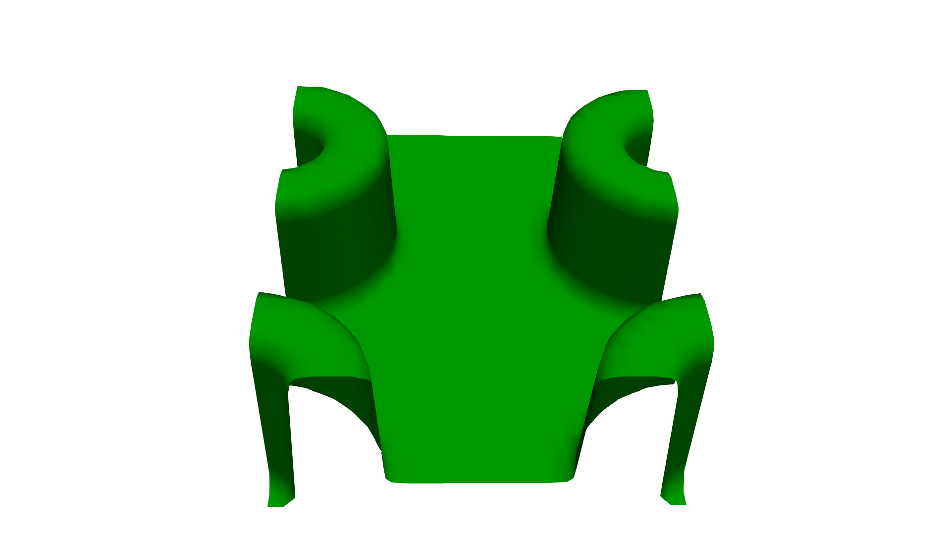
The Quad-Hole example is also based on a process TCAD simulation [62]. The interface domain has four regions of interest, two half holes and two quarter holes (cf. Figure 6.12a). This example is also analyzed in [62], where the example with 48 blocks corresponds to Level 1 and the example with 303 blocks to Level 2.

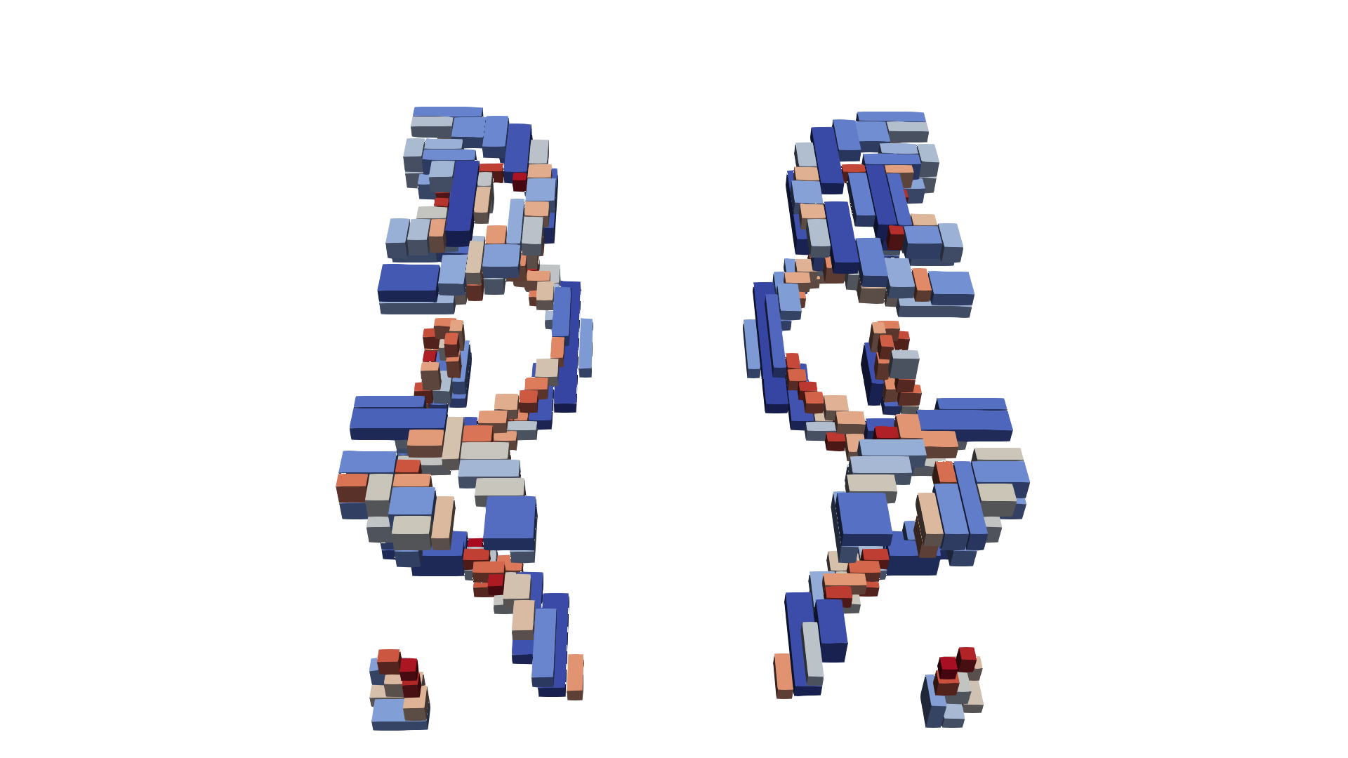
The only block on Level 0 has a size of \(38\times 28\times 30\). There are 48 blocks on Level 1, with their sizes ranging from \(12\times 16\times 12\) to \(68\times 20\times 52\). Their placement is shown in Figure 6.12b. They cover the regions around the quad holes completely. On Level 2 there are 303 blocks, with their sizes ranging from \(12\times 12\times 12\) to \(164\times 20\times 12\) and their placement is shown in Figure 6.12c. They cover only the regions at the top and bottom of the quad holes where there are sharp edges.

The presentation of the results for the Setup FMM is omitted, because the results are qualitatively the same to the ones obtained in the Mandrel example. No new insights are provided: The decomposition introduces a run-time overhead, if only a single thread is used, but by using a higher number of threads the increased parallel efficiency outperform the approach without decomposition.

The single-threaded run-time on Level 0 with a block size and stride width of \(10\,000\) is 0.0013 s. For comparison, the single-threaded run-time with the same parameters on Level 1 is 0.402 s (30 times as long as Level 0) and on Level 2 is 1.568 s (120 times as long as Level 0). Thus, the discussion of Level 0 is skipped.

FMM Level 1

Figure 6.13 shows the gathered run-time data for Level 1. The peak serial speedup of 1.14 is achieved for a stride width of 3.5 and a block size of 75. The serial speedup decreases with smaller block sizes, because of growing overhead introduced by the data exchange between blocks.

Considering parallelization, a stride width between two and 10 is beneficial for the run-time for less than eight threads. The best performance is typically achieved with a stride width of five. The worst performance is achieved with the stride width of 0.5 in almost all cases (except block size 10 and using less than four threads). For a high number of threads, e.g., 24 threads, the maximum stride width performs best. The overall peak performance is achieved with a block size of 50 using 24 threads.

The impact of the block decomposition on the parallel speedup is clear when the best parallel speedup without the developed decomposition (speedup of 8.2) is compared to the best parallel speedup when the developed decomposition is used (speedup of 12.5). Utilizing the second processor does not give any additional performance.

FMM Level 2

On Level 2 the total run-time (cf. Figure 6.14) is four times as high as on Level 1, thus a speedup here has a bigger impact on the overall level-set simulation. Again, a serial speedup of up to 1.05 is observed, for a stride width between two and five, for smaller block sizes the serial speedup declines. Beginning with block size 30 a serial slowdown is measured, again due to the growing overhead introduced by the data exchange between blocks. The peak parallel speedup of 16.6 is achieved for a block size of 75 and a stride width of 20 on Level 2. Comparing the parallel speedup of the block decomposed FMM to the non-decomposed parallel speedup (which reaches 16.5) shows that for an already high number of blocks the decomposition barely effects the performance. The performance only deteriorates in cases with a very small block size (less than 20) where many sub-blocks are created. This is due to the additional overhead created by the synchronization of the sub-blocks.

6.4 Summary

This chapter presented a block decomposition to increase the parallel performance of the FMM on a hierarchical grid. The block decomposition is applicable to all levels of a hierarchical grid yielding a unified parallelization approach. The limited parallel speedup (caused by load-imbalances) of the multi-block FMM on the given blocks of a hierarchical grid are overcome by a novel decomposition strategy. The decomposition strategy splits the given blocks based on a threshold value (block size) into smaller sub-blocks. Thus, the total block count is increased, enabling the control of the number of blocks used in the multi-block FMM. The number of enforced data exchange steps between the blocks based on another parameter (stride width) is evaluated on a hierarchical grid. s The performance of the proposed block decomposition and the parameter values (block size and stride width) is evaluated using three examples. For the generic point source example (a typical test case for benchmarking Eikonal equation solvers) a parallel speedup of 19.1 is achieved using 24 threads. For interface geometries based on process TCAD simulations, speedups of 17.4 for 24 threads are achieved. The original approach without block decomposition achieved a parallel speedup of only 7.4, which is not even half the parallel speedup obtained with the block decomposition. As was shown, the block size shall not be chosen smaller than 30, because for smaller block sizes the overhead usually deteriorate the performance.

The stride width should be chosen between 2.5 and 10 for less than eight threads for best performance, because on a hierarchical grid this reduces the unwanted computations from ghost cell sources. For more than eight threads the maximum stride width (not introducing any additional data exchanges) performs best (shortest run-time), because the computational load between two data exchanges is insufficient otherwise little (the additional synchronization overhead is bigger than the gained performance due to parallelism).