Chapter 6
Adaptive Variable-Order SHE
The structural properties discussed in Chap. 4 show that in the case of spherical energy bands
the coupling between the SHE equations is sparse. This allows for a reduction of memory
requirements for the system matrix of the discretized equations from  to
to  . The
proposed matrix compression scheme further reduces the memory requirements for the system
matrix to
. The
proposed matrix compression scheme further reduces the memory requirements for the system
matrix to  , which finally results in the total memory requirements being dominated
by the
, which finally results in the total memory requirements being dominated
by the 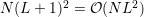 unknowns already at an expansion order of five. For a
three-dimensional device simulation using
unknowns already at an expansion order of five. For a
three-dimensional device simulation using  discrete total energies and
  grid points
(
grid points
( ), the number of unknowns for a first-order expansion are up to
  , where
 even-order expansion coefficients enter the linear solver. On the same grid, a
ninth-order expansion leads to a total of
even-order expansion coefficients enter the linear solver. On the same grid, a
ninth-order expansion leads to a total of  unknowns, of which
  enter
the linear solver. Even though the matrix compression scheme ensures that the total
memory requirements stay within a reasonable amount of a few gigabytes, the high
computational effort due to the large number of unknowns leads to long simulation
times.
enter
the linear solver. Even though the matrix compression scheme ensures that the total
memory requirements stay within a reasonable amount of a few gigabytes, the high
computational effort due to the large number of unknowns leads to long simulation
times.
With the use of unstructured grids for the SHE method as described in Chap. 5, the number
of grid points in the  -space can be reduced to lower numbers than for structured grids
without sacrificing accuracy in critical device regions. Therefore, the total number of unknowns in
the linear system is reduced from
-space can be reduced to lower numbers than for structured grids
without sacrificing accuracy in critical device regions. Therefore, the total number of unknowns in
the linear system is reduced from  to
to  , where
  and
and  refer to the
number of unknowns in
refer to the
number of unknowns in  -space and
  can be a factor two to five smaller than
  ,
cf. Sec. 5.4.
,
cf. Sec. 5.4.
Similar to unstructured grids, which allow for a high resolution in critical regions and a lower
resolution in less important regions, a higher expansion order can be chosen at locations and
energies with high influence on a target quantity such as current, carrier density, or average
carrier velocity. Consequently, instead of a fixed-order expansion as in (2.41), variable-order
expansions of the form
 are
considered in this chapter. The aim is to further reduce the total number of unknowns to
are
considered in this chapter. The aim is to further reduce the total number of unknowns to
 , where the average expansion order
  for a grid point
  obtained by averaging
all positive expansion orders over all positive discrete kinetic energies can be well below an
equivalent uniform expansion order
obtained by averaging
all positive expansion orders over all positive discrete kinetic energies can be well below an
equivalent uniform expansion order  without sacrificing accuracy.
6.1 Variable-Order SHE
The advantage of the SHE method is that the equilibrium distribution is described exactly by a
zeroth-order expansion. This is in contrast to macroscopic transport models derived from
moments of the BTE, where higher-order moments do not vanish. Therefore, it is reasonable to
expect that for the resolution of small deviations from the equilibrium distribution,
only a low expansion order is required for the SHE method in order to obtain good
accuracy.
In this section the discretization of the SHE equations using variable-order expansions is
presented. For a maximum expansion order  in the simulation domain, a variable-order
expansion can be obtained by assembling a system matrix for maximum expansion
order
in the simulation domain, a variable-order
expansion can be obtained by assembling a system matrix for maximum expansion
order  and then imposing homogeneous Dirichlet conditions on all expansion
coefficients
and then imposing homogeneous Dirichlet conditions on all expansion
coefficients  with
with  . However, such an approach is impractical
due to the unnecessary effort of setting up a much larger system matrix than actually
required. In addition, the benefit of reduced memory required for variable expansion orders
is eliminated when setting up a system matrix for uniform expansion order
. However, such an approach is impractical
due to the unnecessary effort of setting up a much larger system matrix than actually
required. In addition, the benefit of reduced memory required for variable expansion orders
is eliminated when setting up a system matrix for uniform expansion order  first.
It is assumed that the unknowns are enumerated in such a way that the expansion coefficients
for a particular box  or a dual box
  are consecutive. In addition, the unknowns
associated with boxes
are consecutive. In addition, the unknowns
associated with boxes  are enumerated first, then the unknowns associated with the dual
boxes
are enumerated first, then the unknowns associated with the dual
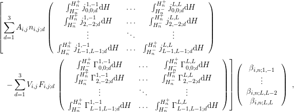
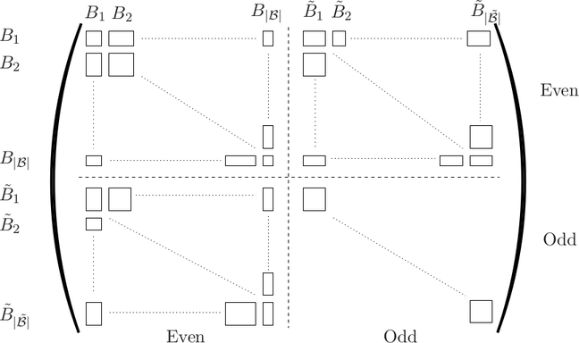
boxes  , which leads to the system matrix structure discussed in Sec. 4.3. The resulting
structure of the system matrix for a uniform expansion order is depicted in Fig. 6.1. The block
sizes for each block coupling two boxes are:
, which leads to the system matrix structure discussed in Sec. 4.3. The resulting
structure of the system matrix for a uniform expansion order is depicted in Fig. 6.1. The block
sizes for each block coupling two boxes are:
Here,  and
and  denote the number of even and odd expansion coefficients up to and
including order
denote the number of even and odd expansion coefficients up to and
including order  respectively. For instance, consider the block in the rows for box
  and in
the columns for the dual box
and in
the columns for the dual box  , which is located at the interface between
  and
and  . From
the discrete equations for the even-order projections in steady-state (5.9) one obtains the system
matrix block for a certain discrete energy
. From
the discrete equations for the even-order projections in steady-state (5.9) one obtains the system
matrix block for a certain discrete energy  directly from rewriting the discrete equations in
matrix form:
directly from rewriting the discrete equations in
matrix form:
 | (6.2) |
where the subscript index  denotes the
  -th component of the vector and the expansion order
 is odd. The matrix block
  results from the scattering operator and is diagonal up to
couplings induced by energy displacements
results from the scattering operator and is diagonal up to
couplings induced by energy displacements  due to inelastic scattering mechanisms,
cf. Thm. 3. A similar structure is obtained for the even-to-even, the odd-to-even, and the
odd-to-odd block.
due to inelastic scattering mechanisms,
cf. Thm. 3. A similar structure is obtained for the even-to-even, the odd-to-even, and the
odd-to-odd block.
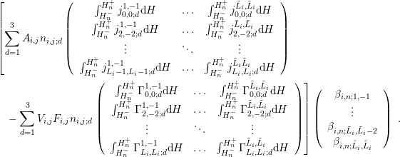
When allowing variable-order expansions, the dimensions of the coupling blocks can differ for
each box  and each dual box
  . Reconsidering the example of the matrix block for the box
 and the dual box
  from above, and assuming an even expansion order
  for
for  and an
odd expansion order
and an
odd expansion order  for the dual box
  , the discrete system of equations is given
by
, the discrete system of equations is given
by
 | (6.3) |
This leads to the system matrix structure shown in Fig. 6.2, where the individual small blocks
are now of different dimension according to the respective expansion order.
The expansion orders for the boxes  and the dual boxes
  should not be
chosen arbitrarily. Consider the case of spherical energy bands, where only a single box
should not be
chosen arbitrarily. Consider the case of spherical energy bands, where only a single box
 carries the maximum even expansion order
  . If all surrounding dual boxes
carry an odd expansion order of at most
. If all surrounding dual boxes
carry an odd expansion order of at most  , then the highest-order expansion
coefficients
, then the highest-order expansion
coefficients  for the box
  do not couple due to Thm. 2 with expansion
coefficients of lower order. Since the right hand side of the linear equation is zero except
for Dirichlet boundary values, the expansion coefficients
do not couple due to Thm. 2 with expansion
coefficients of lower order. Since the right hand side of the linear equation is zero except
for Dirichlet boundary values, the expansion coefficients  are computed as
zero. Moreover, since the size of the final linear system of equations is determined
by the expansion orders of the boxes
are computed as
zero. Moreover, since the size of the final linear system of equations is determined
by the expansion orders of the boxes  only, Thm. 2 suggests that the odd
expansion order of the dual box
only, Thm. 2 suggests that the odd
expansion order of the dual box  should be larger than the even expansion orders
of the two overlapped boxes
should be larger than the even expansion orders
of the two overlapped boxes  and
and  , otherwise the linear system of equations
yields a less accurate solution at the same computational effort. Summing up, one
obtains:
, otherwise the linear system of equations
yields a less accurate solution at the same computational effort. Summing up, one
obtains:
Conversely, since odd expansion orders larger than required do not lead to higher accuracy
because of the same reasoning with the roles of  and
and  exchanged, the odd expansion order
of a dual box is set to the maximum even expansion order of the overlapped boxes plus one,
i.e.
exchanged, the odd expansion order
of a dual box is set to the maximum even expansion order of the overlapped boxes plus one,
i.e.

Consider two neighboring boxes  and
and  with expansion orders
  and
and  ,
,
 . Denote the dual box overlapping
  and
and  with
with  . From Thm. 2 and
Guideline 2 it follows that the expansion coefficients defined for
. From Thm. 2 and
Guideline 2 it follows that the expansion coefficients defined for  couple with expansion
coefficients in
couple with expansion
coefficients in  up to order
  . These expansion coefficients in
  couple
according to Thm. 2 with expansion coefficients in
couple
according to Thm. 2 with expansion coefficients in  up to order
  , thus
there is no gain in accuracy for
, thus
there is no gain in accuracy for  larger than
  . This leads to the second
guideline:
. This leads to the second
guideline:
Guideline 2. The maximum even expansion order of neighboring boxes  and
and  should not differ by more than two.
6.2 Adaptive Control of the SHE Order
In the previous section the efficient assembly of SHE equations using variable expansion orders
has been discussed. However, the variable expansion orders were assumed to be given for each box
 and each dual box
  . For every-day TCAD purposes, such a selection should be based on an
adaptive strategy until a prescribed accuracy for a certain target quantity is reached. This section
thus discusses strategies to automatically pick suitable expansion orders within the simulation
domain. Due to Guideline 1, it suffices to select expansion orders for the the boxes in
. For every-day TCAD purposes, such a selection should be based on an
adaptive strategy until a prescribed accuracy for a certain target quantity is reached. This section
thus discusses strategies to automatically pick suitable expansion orders within the simulation
domain. Due to Guideline 1, it suffices to select expansion orders for the the boxes in
 .
.
What is considered to be a suitable or good expansion order for a box  clearly depends on
the target quantity. Macroscopic quantities are typically obtained by moments of the distribution
function such as
clearly depends on
the target quantity. Macroscopic quantities are typically obtained by moments of the distribution
function such as
 where
where  is a suitable polynomial of
  . Due to the asymptotically exponential decay of the
distribution function
. Due to the asymptotically exponential decay of the
distribution function  with the modulus of
  , the distribution function needs to be computed
with high accuracy at low energies, while lower accuracy is sufficient at higher energies for the
computation of
, the distribution function needs to be computed
with high accuracy at low energies, while lower accuracy is sufficient at higher energies for the
computation of  . However, for the investigation of high-energy phenomena such as hot carrier
degradation [101, 9], the distribution function needs to be fairly accurate at high energies, while
there is less emphasis on accuracy at lower energies. Consequently, suitable expansion orders
depend on the quantities of interest.
. However, for the investigation of high-energy phenomena such as hot carrier
degradation [101, 9], the distribution function needs to be fairly accurate at high energies, while
there is less emphasis on accuracy at lower energies. Consequently, suitable expansion orders
depend on the quantities of interest.
In the following, three different strategies for the adaptive choice of expansion orders are
presented. The first approach is based on an analytical result for the SHE of a function
 in dependence of the smoothness of
  . The second approach increases the
expansion order particularly in regions with high weight on one or more target quantities.
The third approach is a rather classical residual-based technique, which is common in
finite element and finite volume methods [1, 8, 56]. Even though the three strategies
are presented separately, in practice they should be combined in order to obtain best
results.
. The second approach increases the
expansion order particularly in regions with high weight on one or more target quantities.
The third approach is a rather classical residual-based technique, which is common in
finite element and finite volume methods [1, 8, 56]. Even though the three strategies
are presented separately, in practice they should be combined in order to obtain best
results.
6.2.1 Rate of Decay of Expansion Coefficients
The SHE can be seen as the three-dimensional extension of Fourier series. Since the latter is more
widely known than the former, the motivation for the adaptive strategy for SHE is first given for
Fourier series. The transition from Fourier series to SHE does not impose additional
complications then.
A  -periodic function
  can be expanded into trigonometric functions as
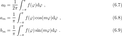
 where
where  . The function
  does not need to be continuous, it is sufficient for
  to be
integrable. The expansion coefficients are computed from
to be
integrable. The expansion coefficients are computed from  as
as
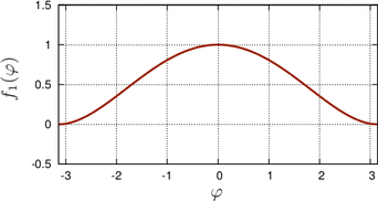
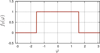
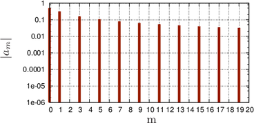
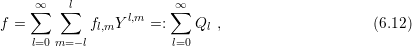
 Consider the two
  -periodic functions depicted in Fig. 6.3
![{
2 4 4 4 2 2 1, |φ| ≤ π∕2 ,
f1(φ ) = [(x− π )(x + π)] ∕π = x ∕π − 2x ∕π + 1 , f2(φ ) = 0, π ∕2 < |φ| ≤ π .
(6.10)](diss-et1300x.png) While
While  is continuously differentiable,
  is discontinuous. The Fourier series of the functions
are given by
is discontinuous. The Fourier series of the functions
are given by
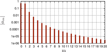
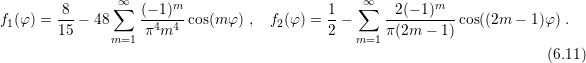 For
the smooth function
For
the smooth function  , the Fourier coefficients decay with the fourth power of
  , while the
Fourier coefficients of
, while the
Fourier coefficients of  only decay inversely proportional to
  . More generally,
it can be shown that for a function with integrable derivatives up to order
. More generally,
it can be shown that for a function with integrable derivatives up to order  , the
expansion coefficients decay at least with rate
, the
expansion coefficients decay at least with rate  . Conversely, the rate of decay of
the Fourier coefficients are a measure for the smoothness of the expanded function
[28, 13].
. Conversely, the rate of decay of
the Fourier coefficients are a measure for the smoothness of the expanded function
[28, 13].
For SHE, a similar result holds for a function  defined on the unit sphere
  [31, 18]:
Since the spherically symmetric distribution function  in equilibrium is described exactly by
a zeroth-order expansion, higher-order expansion coefficients provide a measure for the distortion
of
in equilibrium is described exactly by
a zeroth-order expansion, higher-order expansion coefficients provide a measure for the distortion
of  from equilibrium. This is in contrast to macroscopic models derived from moments of the
BTE such as those described in Sec. 1.1, where even moments of the distribution function in
equilibrium do not vanish.
from equilibrium. This is in contrast to macroscopic models derived from moments of the
BTE such as those described in Sec. 1.1, where even moments of the distribution function in
equilibrium do not vanish.
Given a numerical solution of the SHE equations for certain expansion orders  , an
adaptive adjustment of the expansion order can be based on (6.13). Division by
, an
adaptive adjustment of the expansion order can be based on (6.13). Division by  and
taking the logarithm leads for
and
taking the logarithm leads for  to
to
 where here and in the following
  refers to
 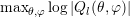 . Taking the left hand
side as an estimate for
. Taking the left hand
side as an estimate for  and dropping the constant
  , which acts only as an offset to the
estimate on the rate of decay
, which acts only as an offset to the
estimate on the rate of decay  , results in
 with
with
 taking the role of an error estimator. The larger the value of
  at a certain point
  ,
the slower is the decay of the distribution function, thus the higher is the expected gain in
accuracy from an increased expansion order.
,
the slower is the decay of the distribution function, thus the higher is the expected gain in
accuracy from an increased expansion order.
Since due to Guideline 1 the highest available expansion order is associated with dual boxes in
 , the rate of decay for a box
  can be based either on the highest expansion order for the
box
can be based either on the highest expansion order for the
box  , or on the dual boxes
  overlapping
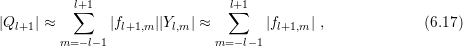
  . In the latter case, one obtains for the error
estimator
. In the latter case, one obtains for the error
estimator  for the box
![[∑ ]
B˜i,j log |Ql+1 |
ηi ∼ ------N˜-------− log f0,0 ∕log(l + 1) , (6.16)
i](diss-et1346x.png) where the maximum expansion order in
where the maximum expansion order in  is
is  , the sum extends over the dual boxes
overlapping
, the sum extends over the dual boxes
overlapping  and
and  denotes the number of dual boxes overlapping
  .
.
The exact evaluation of the the term  is a maximization
problem over all angles and leads to high overall numerical effort, because such a maximization
problem needs to be solved at every grid point
is a maximization
problem over all angles and leads to high overall numerical effort, because such a maximization
problem needs to be solved at every grid point  . A numerically very cheap
approximation to the maximum is
. A numerically very cheap
approximation to the maximum is
 since
the expansion coefficients
since
the expansion coefficients  are readily available. The approximation
  leads to an
overestimation of the maximum, but is not a concern because it leads to a constant offset in the
error indicator
leads to an
overestimation of the maximum, but is not a concern because it leads to a constant offset in the
error indicator  only.
only.
The case  in (6.16) requires additional treatment since
  evaluates
to zero. Replacing
evaluates
to zero. Replacing  by
by  resolves these problems and partly accounts for the
overestimation of
resolves these problems and partly accounts for the
overestimation of  by (6.17). For larger values of
  , the replacement of
  by
by
 does not cause a significant difference anyway. This leads to the final form of the
estimator:
does not cause a significant difference anyway. This leads to the final form of the
estimator:
![[∑ ˜ log[∑Li+1 |fL+1,m(B˜i,j)|] ]
ηi ∼ ---Bi,j------m=−-Li−-1---i---------- − log |f0,0| ∕log(Li + 2) , (6.18)
N˜i](diss-et1366x.png) where
where  denotes the maximum even expansion order of the box
  . After an evaluation of the
estimator for all boxes
. After an evaluation of the
estimator for all boxes  , the expansion order can then be increased for the boxes with largest
values of
, the expansion order can then be increased for the boxes with largest
values of  . An additional smoothing step then ensures conformity with respect to Guidelines 1
and 2.
. An additional smoothing step then ensures conformity with respect to Guidelines 1
and 2.
The estimator (6.18) is based on the rate of decay of the expansion coefficients only and does
not consider the exponential decay of the distribution function at higher energies. Therefore, the
estimator treats regions with large values of the distribution function as being equally important
as regions with very low values of the distribution function. This is a disadvantage if the
target quantity is a macroscopic quantity such as the average carrier velocity, for which
only large values of the distribution function lead to significant contributions. In such
situations, an additional term  may be added to (6.18) in order to penalize
low-probability regions of the distribution function. In the special case
may be added to (6.18) in order to penalize
low-probability regions of the distribution function. In the special case 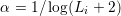 , this
modification is equivalent to dropping the term
, this
modification is equivalent to dropping the term  from (6.18). It should be
noted that this modification towards higher weight at regions with high probability is
similar in spirit to a target quantity driven control of the expansion order discussed
next.
from (6.18). It should be
noted that this modification towards higher weight at regions with high probability is
similar in spirit to a target quantity driven control of the expansion order discussed
next.
6.2.2 Target Quantity Driven Adaptive Control
Another approach to the adaptive control of the expansion order is based on one or more
dedicated target quantities, for which the expansion orders are chosen such that a prescribed
accuracy is obtained. For instance, consider as target quantity the average particle
energy
 The
average energy of a discrete solution
The
average energy of a discrete solution  of the SHE equations is computed using e.g. a
simple midpoint quadrature rule as
of the SHE equations is computed using e.g. a
simple midpoint quadrature rule as
 Hence, this allows for an extraction of the individual weight
  of the grid node
 on the target quantity as
 Weights for other target quantities such as the average carrier velocity or the carrier density can
be defined in a similar manner. Therefore,
Weights for other target quantities such as the average carrier velocity or the carrier density can
be defined in a similar manner. Therefore,  can be seen as a generic weight function for
an arbitrary target quantity
can be seen as a generic weight function for
an arbitrary target quantity  , where typically macroscopic target quantities of the form
 are of interest.
An increase of the expansion order is most appropriate in regions where the weights  are
high. On the contrary, regions with a weight of several orders of magnitude below the boxes of
highest weight can be kept at lowest expansion order, because the contribution to the target
quantity is very small anyway.
are
high. On the contrary, regions with a weight of several orders of magnitude below the boxes of
highest weight can be kept at lowest expansion order, because the contribution to the target
quantity is very small anyway.
A comparison of the weight functions for the calculation of the average carrier energy of a
Maxwellian distribution  and a shifted and heated Maxwellian distribution
  is depicted in
Fig. 6.4. For the Maxwellian distribution it is sufficient to consider only energies up to about
is depicted in
Fig. 6.4. For the Maxwellian distribution it is sufficient to consider only energies up to about  eV for the computation of the average energy at an accuracy of about one percent, because the
weights at higher energies are below
eV for the computation of the average energy at an accuracy of about one percent, because the
weights at higher energies are below  already. However, for the shifted and heated
Maxwellian distribution, contributions up to an energy of about
already. However, for the shifted and heated
Maxwellian distribution, contributions up to an energy of about  eV need to be considered
for comparable accuracy.
eV need to be considered
for comparable accuracy.
6.2.3 Residual-Based Adaptive Control
An expansion order control based solely on the weight function  does not account
appropriately for long-range influences of regions of the distribution function with low probability
on regions with higher probability. This is a particular concern in short devices at high electric
fields, where strong variations of the distribution function with respect to energy are observed.
Similar to the estimation of the rate of decay in Sec. 6.2.1, a residual-based approach provides a
better monitor for the need for higher expansion orders than the target quantity driven approach
in the previous section.
does not account
appropriately for long-range influences of regions of the distribution function with low probability
on regions with higher probability. This is a particular concern in short devices at high electric
fields, where strong variations of the distribution function with respect to energy are observed.
Similar to the estimation of the rate of decay in Sec. 6.2.1, a residual-based approach provides a
better monitor for the need for higher expansion orders than the target quantity driven approach
in the previous section.
Let  denote the numerical solution of the SHE equations for a
possibly variable expansion order
denote the numerical solution of the SHE equations for a
possibly variable expansion order  obtained from the solution of the
system
obtained from the solution of the
system
 Now,
let
Now,
let  denote the prolongated solution
  for a possibly variable
expansion order
for a possibly variable
expansion order  obtained by
 Denoting the system matrix for the expansion orders
  with
with  and the right hand side with
 , the residual
 provides an indication on where to increase the expansion order. In order to make the
residual invariant with respect to the scale of the values
provides an indication on where to increase the expansion order. In order to make the
residual invariant with respect to the scale of the values  , the linear system
should be first symmetrized and rescaled as discussed in Sec. 7.2. Note that the matrix
compression scheme derived and discussed in Chap. 4 allows for a convenient means to store
the larger system matrix
, the linear system
should be first symmetrized and rescaled as discussed in Sec. 7.2. Note that the matrix
compression scheme derived and discussed in Chap. 4 allows for a convenient means to store
the larger system matrix  and to compute the matrix-vector product
  efficiently.
It is important to keep in mind that the residual is not invariant with respect to
transformations of the linear system. In particular, if the  -th equation is multiplied with a
certain factor, then also the residual is multiplied with the same factor, even though the solution
of the linear system is unchanged. Consequently, it is advisable to first apply normalizations, for
instance by multiplication of each equation in the system with the reciprocal of the respective
diagonal entry.
-th equation is multiplied with a
certain factor, then also the residual is multiplied with the same factor, even though the solution
of the linear system is unchanged. Consequently, it is advisable to first apply normalizations, for
instance by multiplication of each equation in the system with the reciprocal of the respective
diagonal entry.
Similar to other expansion order control strategies outlined above, an increase of the
expansion order can finally be carried out for boxes with highest residuals. An additional
expansion order smoothing step after the increase ensures that Guidelines 1 and 2 are
obeyed.
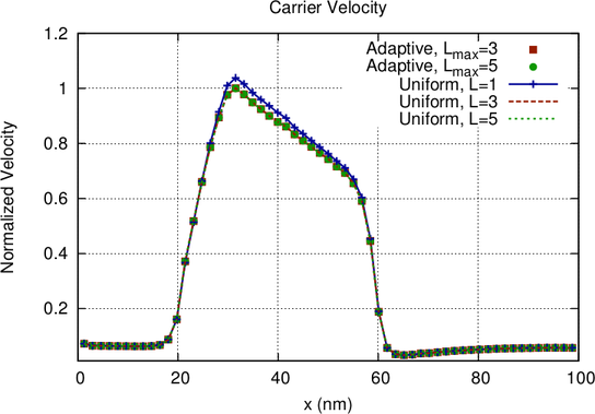
6.3 Results
Average carrier velocities along a  nm
nm  -diode with a bias of
  Volt and intrinsic
region between
Volt and intrinsic
region between  nm and
  nm are compared for different uniform expansion orders
as well as for the three adaptive expansion order schemes after one (maximum SHE order 3), two
(maximum SHE order 5) and three (maximum SHE order 7) adaption steps. The total energy
range spans
nm are compared for different uniform expansion orders
as well as for the three adaptive expansion order schemes after one (maximum SHE order 3), two
(maximum SHE order 5) and three (maximum SHE order 7) adaption steps. The total energy
range spans  eV using an energy spacing of
  meV. A first-order expansion is kept directly
at the band edge, because it has been observed that it improves numerical stability at high
expansion orders. At the contacts, a Maxwell distribution is imposed as a Dirichlet boundary
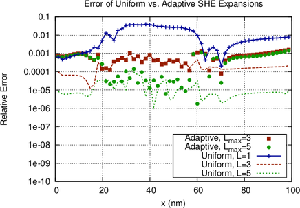
condition, thus the expansion is kept at first order there. The resulting velocity curves are
depicted in Fig. 6.5 and show rather small differences between the different expansion
orders. Nevertheless, the logarithmic plots of the relative errors in Fig. 6.9 provide full
insight.
meV. A first-order expansion is kept directly
at the band edge, because it has been observed that it improves numerical stability at high
expansion orders. At the contacts, a Maxwell distribution is imposed as a Dirichlet boundary
condition, thus the expansion is kept at first order there. The resulting velocity curves are
depicted in Fig. 6.5 and show rather small differences between the different expansion
orders. Nevertheless, the logarithmic plots of the relative errors in Fig. 6.9 provide full
insight.
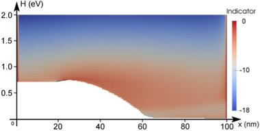
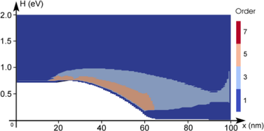
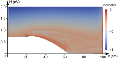
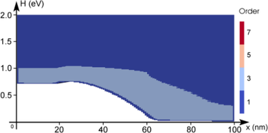
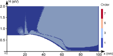
The adaptive strategy based on the decay of expansion coefficients as described in Sec. 6.2.1
is illustrated in Fig. 6.6. In order to emphasize refinement in high-probability regions, the
term  is added to (6.18) as discussed above. The resulting indiciator
values are shifted such that the highest value is zero. The threshold for an expansion
order increase is set to
is added to (6.18) as discussed above. The resulting indiciator
values are shifted such that the highest value is zero. The threshold for an expansion
order increase is set to  . The indicator is not computed at the contact, but
evaluated to
. The indicator is not computed at the contact, but
evaluated to  in Fig. 6.6. During the adaption procedure, the adaptive control stays at a
first-order expansion in the left
in Fig. 6.6. During the adaption procedure, the adaptive control stays at a
first-order expansion in the left  region, where the distribution function is still close to
equilibrium. The expansion order is then increased in the intrinsic region and away
from the band edge at higher energies after the intrinsic regions. In summary, the
adaptive strategy based on the decay of the expansion coefficients increases the expansion
order mostly along the high energy tail and close to the band edge inside the intrinsic
region. The increase of the expansion order near the right contact stems from the use of
Dirichlet boundary conditions and can be considered to be an artifact, because the
distribution function is forced from a heated distribution to a Maxwell distribution at
the contact, leading to an unphysical boundary layer as discussed by Schroeder et al.
[92].
region, where the distribution function is still close to
equilibrium. The expansion order is then increased in the intrinsic region and away
from the band edge at higher energies after the intrinsic regions. In summary, the
adaptive strategy based on the decay of the expansion coefficients increases the expansion
order mostly along the high energy tail and close to the band edge inside the intrinsic
region. The increase of the expansion order near the right contact stems from the use of
Dirichlet boundary conditions and can be considered to be an artifact, because the
distribution function is forced from a heated distribution to a Maxwell distribution at
the contact, leading to an unphysical boundary layer as discussed by Schroeder et al.
[92].
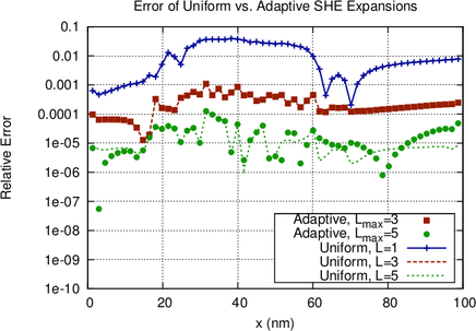
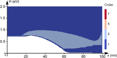
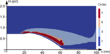
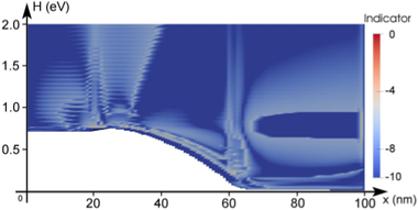
A different behavior is observed for the target quantity based control shown in
Fig. 6.7. The indicator is obtained by taking the logarithm of the contribution of the
respective box in the simulation domain and shifting the values such that the highest
contribution leads to an indicator value of zero. A threshold value of  has been
used for increasing the expansion order. Since the distribution function changes its
shape only mildly at higher energies, the indicator is essentially unchanged during the
adaption, leading to higher expansion orders near the band edge only. Note that the
high-energy tail of the distribution function right after the intrinsic region is resolved by
the increased expansion order. The error plot in Fig. 6.9(b) shows that virtually the
same accuracy as for uniform expansions is obtained. However, the expansion order at
later adaption steps abruptly changes from first-order to highest order as quickly as
possible without violating Guidelines 1 and 2, thus it is reasonable to expect that a less
abrupt change of the expansion order can preserve the accuracy using a lower number of
unknowns.
has been
used for increasing the expansion order. Since the distribution function changes its
shape only mildly at higher energies, the indicator is essentially unchanged during the
adaption, leading to higher expansion orders near the band edge only. Note that the
high-energy tail of the distribution function right after the intrinsic region is resolved by
the increased expansion order. The error plot in Fig. 6.9(b) shows that virtually the
same accuracy as for uniform expansions is obtained. However, the expansion order at
later adaption steps abruptly changes from first-order to highest order as quickly as
possible without violating Guidelines 1 and 2, thus it is reasonable to expect that a less
abrupt change of the expansion order can preserve the accuracy using a lower number of
unknowns.
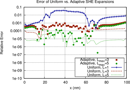
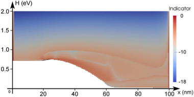
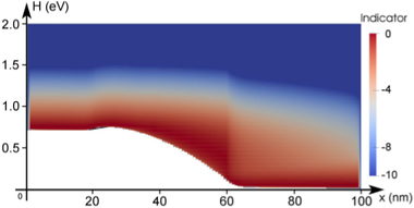
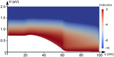
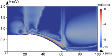
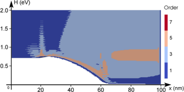
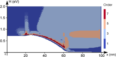
Fig. 6.8 depicts the effect of the residual based expansion order control. The residual has been
normalized first by scaling the uniform system such that a unit diagonal is obtained. The
indicator is then obtained by taking the logarithm of the residual values and applying a suitable
shift such that the highest residual value leads to an indicator value of zero. The expansion order
is increased if the indicator is larger than  . In principle, one may assign less weight to
higher energies such as for the adaptive strategy based on the rate of decay of expansion
coefficients. For illustration purposes, the unmodified indicator is shown. It should be
noted that the strategy based on the decay leads to qualitatively similar indicator
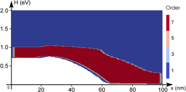
values if no modification at higher energies is applied. The pure residual based strategy
increases the expansion order to third-order up to high energies in the right half of the
device. However, fifth-order expansions are used in a very small region in the device
only. A seventh-order expansion is only assigned right above the band edge inside the
intrinsic region. The error plot in Fig. 6.9(c) is very similar to the error plot for the
strategy based on the decay of expansion coefficients, hence the same conclusions can be
drawn.
. In principle, one may assign less weight to
higher energies such as for the adaptive strategy based on the rate of decay of expansion
coefficients. For illustration purposes, the unmodified indicator is shown. It should be
noted that the strategy based on the decay leads to qualitatively similar indicator
values if no modification at higher energies is applied. The pure residual based strategy
increases the expansion order to third-order up to high energies in the right half of the
device. However, fifth-order expansions are used in a very small region in the device
only. A seventh-order expansion is only assigned right above the band edge inside the
intrinsic region. The error plot in Fig. 6.9(c) is very similar to the error plot for the
strategy based on the decay of expansion coefficients, hence the same conclusions can be
drawn.
Fig. 6.9 further shows that the SHE method converges to a solution as the expansion order
increases. As reference, a uniform seventh-order expansion is used. A first-order expansion shows
an average error of about  over the device with respect to the seventh-order
expansion taken as reference. The average error of a third-order expansion is around
over the device with respect to the seventh-order
expansion taken as reference. The average error of a third-order expansion is around
 , and approximately
  for a fifth-order expansion. A similar exponential
decay of the error with the SHE order has also been observed by Jungemann et al.
[53] for the collector current of a bipolar junction transistor, even though at a lower
rate.
for a fifth-order expansion. A similar exponential
decay of the error with the SHE order has also been observed by Jungemann et al.
[53] for the collector current of a bipolar junction transistor, even though at a lower
rate.
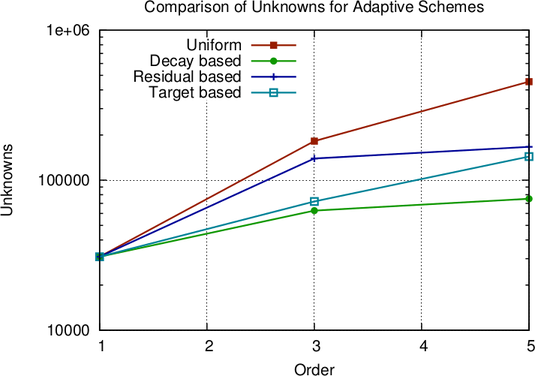
The number of unknowns obtained with uniform and three adaptive expansions are depicted
in Fig. 6.10. Savings of a factor of almost three are obtained with the target quantity based
scheme, which yields virtually the same accuracy as uniform expansions. Memory requirements
and execution times are consequently reduced by the same factor. Typically, higher savings for
the execution times are obtained in practice, because linear solvers with optimal complexity are
not available in general. A combination of the three different schemes proposed may
give slightly higher savings, which become significant at very high expansion orders
only.
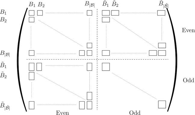
 and
and  do not have a common interface,
the respective blocks are zero. If boxes
do not have a common interface,
the respective blocks are zero. If boxes  and
and  do not overlap, the respective blocks
are also zero. The odd-to-odd coupling implies a diagonal block due to the structure of the
scattering operators.
do not overlap, the respective blocks
are also zero. The odd-to-odd coupling implies a diagonal block due to the structure of the
scattering operators.


 and a
discontinuous function
and a
discontinuous function  .
.


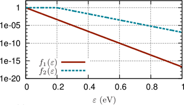
 and a shifted, heated Maxwellian
  . The two weights are normalized to
a peak value
. The two weights are normalized to
a peak value  .
.
 diode for three
adaption steps using an adaptive scheme based on the decay of expansion coefficients as
outlined in Sec.
diode for three
adaption steps using an adaptive scheme based on the decay of expansion coefficients as
outlined in Sec.  .
.

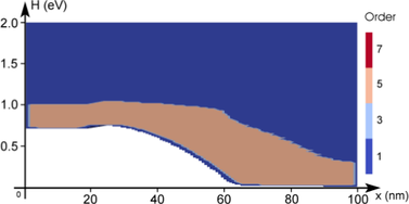
 diode for three
adaption steps using an adaptive scheme based on a target quantity as discussed in
Sec.
diode for three
adaption steps using an adaptive scheme based on a target quantity as discussed in
Sec. 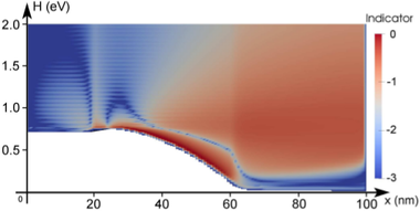
 diode for three
adaption steps using an adaptive scheme based on residuals as described in Sec.
diode for three
adaption steps using an adaptive scheme based on residuals as described in Sec.