 . Consider
Up to now, the SHE equations have been derived and investigated on the continuous level. Generic discretization schemes were considered in the previous chapter and a system matrix compression scheme was developed. It is thus time to consider the discretization of the equations, which is the focus of this chapter. To make the chapter as self-contained as possible, the necessary prerequisites about the box integration scheme and the generation of suitable unstructured grids are presented first.
The box integration scheme is a widely used discretization scheme, particularly for semiconductor device simulation and for fluid dynamics. Outside the field of microelectronics it is typically called finite volume method [4, 64]. The main advantage of the box integration scheme is its local conservation property, thus it is particularly suited for the discretization of conservation equations such as the drift-diffusion equations. The box integration can be derived in different ways. In this section a rather direct approach is taken, while a mathematically cleaner approach can be found in [4], where connections with the finite element method are more pronounced.
In the following, the box integration scheme is explained by example of the discretization of
the Poisson equation on the domain . Consider
| Δψ | = f in Ξ ⊂ ℝn , | ||
| ψ | = 0 on ∂Ξ , |
 of the domain
  into small boxes
  , a local integral form of the Poisson
equation is
, a local integral form of the Poisson
equation is
| ∫ BiΔψdV | = ∫ BifdV on Ξ , ∫ ∂Bi∩∂ΞψdA = 0 . |
| ∫ ∂Bi∇ψ ⋅ndA | = ∫ BifdV on Ξ , ∫ Bi∩∂ΞψdA = 0 , |
 denotes the unit normal vector to the boundary of the box in outward direction.
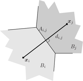
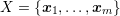
Let the connecting line ![[xi,xj]](diss-et947x.png) of the box centers
of the box centers  and
and  of the boxes
  and
and  be
perpendicular to the box boundary, cf. Fig. 5.1. A first-order approximation of the normal
derivative of the potential is a differential quotient along the connecting line
be
perpendicular to the box boundary, cf. Fig. 5.1. A first-order approximation of the normal
derivative of the potential is a differential quotient along the connecting line ![[xi,xj]](diss-et952x.png) of length
of length
 . Thus, one obtains the discrete local conservation equations
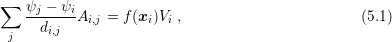
 denotes the volume of the box
  and the interface area
  is zero if the boxes
  and
and  do not have a common boundary. Note that the transition from the continuous to the
discrete formulation requires an approximation of fluxes through the box boundaries. There exists
a large number of different flux approximation schemes, an overview can be found e.g. in the
textbook of LeVeque [64].
do not have a common boundary. Note that the transition from the continuous to the
discrete formulation requires an approximation of fluxes through the box boundaries. There exists
a large number of different flux approximation schemes, an overview can be found e.g. in the
textbook of LeVeque [64].
 and
and  is
is  , while the area of the interface between boxes
  and
and  is
is  .
.
To summarize, the main ingredients of a box integration scheme are as follows:
 of the tessellation
  of
the domain
of
the domain  .
.
Two families of tessellations  of the domain
  are frequently used with a box integration
scheme. The first family is referred to as vertex-centered, where the unknowns and the boxes
are frequently used with a box integration
scheme. The first family is referred to as vertex-centered, where the unknowns and the boxes
 are associated with the vertices of another mesh. The second family is based on a
cell-centered approach, where the unknowns are directly associated with the cells of the mesh
(e.g. triangles, tetrahedra, hexahedra), which also constitute the boxes
are associated with the vertices of another mesh. The second family is based on a
cell-centered approach, where the unknowns are directly associated with the cells of the mesh
(e.g. triangles, tetrahedra, hexahedra), which also constitute the boxes  . Other
formulations such as cell-vertex methods exist [4], but are not further addressed in the
following. The respective preference of a certain family is often based on the availability of
good flux approximation schemes for the problem at hand. Due to the wide-spread
use of vertex-centered box integration schemes in the field of semiconductor device
simulation, the focus in this section is on this first family. In particular, the box integration
scheme for the SHE equations presented in the next section is based on a vertex-centered
construction.
. Other
formulations such as cell-vertex methods exist [4], but are not further addressed in the
following. The respective preference of a certain family is often based on the availability of
good flux approximation schemes for the problem at hand. Due to the wide-spread
use of vertex-centered box integration schemes in the field of semiconductor device
simulation, the focus in this section is on this first family. In particular, the box integration
scheme for the SHE equations presented in the next section is based on a vertex-centered
construction.
While a cell-centered box integration scheme can be carried out on virtually any mesh, the
vertex-centered method is a-priori based on a different mesh and the boxes in  need to be
constructed first. The following two constructions are common [4]:
need to be
constructed first. The following two constructions are common [4]:
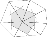
(a) Circumcenter method (Voronoi diagram). |
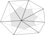
(b) Barycenter method. |
 . Each
box
. Each
box  consists of points closer to
  than to any other point of
  ,
i.e.
,
i.e.

 . Here, a triangulation does not necessarily
refer to a triangulation in two spatial dimensions, but may also refer to the general
case of a decomposition of the
. Here, a triangulation does not necessarily
refer to a triangulation in two spatial dimensions, but may also refer to the general
case of a decomposition of the  -dimensional space into
  -simplices. Note that not
every triangulation is the dual of a Voronoi diagram: If the circumsphere of a cell
-simplices. Note that not
every triangulation is the dual of a Voronoi diagram: If the circumsphere of a cell  includes vertices other than those of
  , then the triangulation is not the dual of a
Voronoi diagram. Triangulations, which are the dual of a Voronoi diagram, are called
Delaunay triangulations. Unlike for the unstructured case, Voronoi diagrams can be
derived directly from structured grids, particularly meshes consisting of rectangles and
bricks.
, then the triangulation is not the dual of a
Voronoi diagram. Triangulations, which are the dual of a Voronoi diagram, are called
Delaunay triangulations. Unlike for the unstructured case, Voronoi diagrams can be
derived directly from structured grids, particularly meshes consisting of rectangles and
bricks.
The advantage of Voronoi diagrams is that the interfaces between boxes are perpendicular to the connections between the respective vertices, thus allowing for the simple approximation of the normal flux. However, the generation of underlying Delaunay triangulations results in additional effort needed for mesh generation on the one hand and mesh refinement on the other hand [94, 113]. In addition, the computation of Voronoi diagrams becomes increasingly challenging in higher spatial dimensions.
In order to employ a box integration scheme, there is usually no need to set up the boxes
explicitly. As motivated in Sec. 5.1, it is usually sufficient to have the box volumes  and the
interface areas
and the
interface areas  available. For the discretization of an additional advective term, the box
volume fraction
available. For the discretization of an additional advective term, the box
volume fraction  associated with the interface
  is also required, cf. Fig. 5.3. Since
the computation of these values for triangular and tetrahedral meshes is only poorly
documented in the relevant literature, the respective algorithms are detailed in the
following.
is also required, cf. Fig. 5.3. Since
the computation of these values for triangular and tetrahedral meshes is only poorly
documented in the relevant literature, the respective algorithms are detailed in the
following.
 is highlighted. The Voronoi volume fraction
  and the
interface area
and the
interface area  are associated with each edge
 ![[xi,xj]](diss-et995x.png)
Since Voronoi quantities are required based on connections between  and
and  , it is
sufficient to provide an algorithm for the computation of the respective quantities for each edge
, it is
sufficient to provide an algorithm for the computation of the respective quantities for each edge
![[xi,xj]](diss-et998x.png) . The Voronoi information for the full domain is then obtained by an iteration over all
edges of the domain.
. The Voronoi information for the full domain is then obtained by an iteration over all
edges of the domain.
Algorithm 3 (Computation of Voronoi quantities for a triangular Delaunay mesh).
Requirements: Triangular Delaunay mesh with all circumcenters in the interior of the mesh
Input: edge ![[xi,xj]](diss-et999x.png)
 and
and  .
.
 and set
  to the midpoint
of the edge.
to the midpoint
of the edge.
 .
.
 .
.
 .
.Return  .
.
The box volumes  for the box associated with vertex
  is obtained by a summation over
all box fractions, i.e.
is obtained by a summation over
all box fractions, i.e.  . The three-dimensional equivalent is slightly more
involved:
. The three-dimensional equivalent is slightly more
involved:
Algorithm 4 (Computation of Voronoi quantities for a tetrahedral Delaunay mesh).
Requirements: Triangular Delaunay mesh with all circumcenters in the interior of the mesh
Input: edge ![[x ,x ]
i j](diss-et1011x.png)
 .
.
 .
.
 .
.
![[xi,xj,xk,xl]](diss-et1015x.png) , compute the circumcenter
, compute the circumcenter  .
.
 , where
  is the number of adjacent cells.
![[xi,xj,xk]](diss-et1019x.png) adjacent to edge
adjacent to edge ![[xi,xj]](diss-et1020x.png) , do
, do
 and
and  denote the two circumcenters.
 and
set
and
set  to the circumcenter of the facet.
 of the triangle
 ![[p,c ,c ]
1 2](diss-et1026x.png) .
.
 .
.
 .
.Return  .
.
Note that the point  is used for the computation of the polygon defined by the
circumcenters. Again, the box volumes
is used for the computation of the polygon defined by the
circumcenters. Again, the box volumes  are obtained by a summation over all
  related to
a vertex
related to
a vertex  .
.
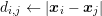
It has to be noted that the Delaunay property does not ensure that the circumcenters of all
cells are inside the mesh, i.e. located inside or at the boundary of any cell of the mesh.
Consequently, cells with regular shapes are required near the mesh boundary in order to fulfill the
requirements of the two algorithms above, cf. Fig. 5.4. If this criterion is not strictly fulfilled, the
system matrix  will be disturbed by, say, a matrix
  . Similar to the analysis of round-off
errors, the difference of the solution
. Similar to the analysis of round-off
errors, the difference of the solution  of the perturbed system with respect to the true solution
 is bounded by

 denotes the condition number of
  and suitable vector and matrix norms are
chosen [27]. Consequently, violations in the range of round-off errors can be justified from a
mathematical point of view. Higher violations are acceptable if the condition number is known to
be small and only low accuracy in the solution vector is required. In practice, however, even much
stronger violations than those justified from the analytical bound (5.3) can result in insignificant
errors in the solution vector due to high regularity of the underlying formation. Nevertheless, the
regularity of the mesh near the boundary is particularly important for semiconductor device
simulations with dominant current flow near the surface, as it is the case e.g. in a
MOSFET.
and suitable vector and matrix norms are
chosen [27]. Consequently, violations in the range of round-off errors can be justified from a
mathematical point of view. Higher violations are acceptable if the condition number is known to
be small and only low accuracy in the solution vector is required. In practice, however, even much
stronger violations than those justified from the analytical bound (5.3) can result in insignificant
errors in the solution vector due to high regularity of the underlying formation. Nevertheless, the
regularity of the mesh near the boundary is particularly important for semiconductor device
simulations with dominant current flow near the surface, as it is the case e.g. in a
MOSFET.
The generation of Delaunay triangulations of good quality for arbitrary domains is a challenging task already in two dimensions [94], and particularly in three dimensions [17]. The meshes used throughout this thesis are generated by Netgen [91], which is capable of generating two- and three-dimensional Delaunay triangulations. A further discussion of the peculiarities of Delaunay mesh generation and refinement is, however, beyond the scope of this thesis.
The SHE method requires an energy coordinate in addition to the spatial coordinate. In
principle, one may generate a mesh directly for the  -space, but this is impractical for two
reasons. First, the author is not aware of the existence any four-dimensional mesh
generators capable of handling complex domains. Second, the essence of the
-space, but this is impractical for two
reasons. First, the author is not aware of the existence any four-dimensional mesh
generators capable of handling complex domains. Second, the essence of the  -transform
in Sec. 2.3 is the possibility to align the grid with the trajectory of electrons in free
flight given by planes of constant total energy
-transform
in Sec. 2.3 is the possibility to align the grid with the trajectory of electrons in free
flight given by planes of constant total energy  . Consequently, the embedding of a
mesh from the spatial domain to the
. Consequently, the embedding of a
mesh from the spatial domain to the  -space by a tensorial prolongation is of
advantage. Given discrete total energies
-space by a tensorial prolongation is of
advantage. Given discrete total energies  , every vertex
  in the
 -dimensional mesh is first embedded in the
  -dimensional space at location
  .
The full
.
The full  -dimensional mesh of prismatic cells is then obtained by repeatedly
shifting the three-dimensional mesh along the energy axis to obtain the points
-dimensional mesh of prismatic cells is then obtained by repeatedly
shifting the three-dimensional mesh along the energy axis to obtain the points  ,
,
 ,
,  ,
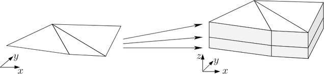
,  . The procedure is illustrated in Fig. 5.5 for the case of
a spatially two-dimensional mesh. Clearly, the energy spacing does not need to be
equidistant. Moreover, the computation of Voronoi quantities for the mesh in
. The procedure is illustrated in Fig. 5.5 for the case of
a spatially two-dimensional mesh. Clearly, the energy spacing does not need to be
equidistant. Moreover, the computation of Voronoi quantities for the mesh in  -space
is obtained from Voronoi information in
-space
is obtained from Voronoi information in  -space by a multiplication of the energy
spacing.
-space by a multiplication of the energy
spacing.
There is no need for setting up the mesh in  -space explicitly, because the additional
 coordinate can also be handled implicitly. Since the coupling of different energy levels is local
in space, it is more memory efficient to stick with the spatial mesh and to store the total
energy values in an array with, say,
coordinate can also be handled implicitly. Since the coupling of different energy levels is local
in space, it is more memory efficient to stick with the spatial mesh and to store the total
energy values in an array with, say,  elements. The respective array index
  can
then be used to identify e.g. the vertex
can
then be used to identify e.g. the vertex  , even though only the vertex
  is
explicitly stored. Since this approach leads to better compatibility with other macroscopic
transport models, which do not require an additional energy coordinate, this implicitly
tensorial representation is used in ViennaSHE. The price to pay is an additional effort
required for for a visualization of the computed distribution function in one and two
spatial dimensions, because the mesh in
is
explicitly stored. Since this approach leads to better compatibility with other macroscopic
transport models, which do not require an additional energy coordinate, this implicitly
tensorial representation is used in ViennaSHE. The price to pay is an additional effort
required for for a visualization of the computed distribution function in one and two
spatial dimensions, because the mesh in  -space needs to be made available
then.
-space needs to be made available
then.
With the discussion of the box integration scheme in Sec. 5.1 and the computation of Voronoi information from Sec. 5.2, the discretization of the SHE equations (2.34) and (2.35) can now be tackled. For the sake of clarity, the SHE method for spherical energy bands in steady-state is considered. The general case is obtained without additional difficulties.
Due to the use of MEDS for stabilization, cf. Sec. 2.3, two different sets of equations (2.34)
and (2.35) need to be considered. The even-order equations are discretized directly on the boxes
 of the underlying Voronoi tessellation
  , while the odd-order equations are associated with
the dual tessellation
, while the odd-order equations are associated with
the dual tessellation  centered at the interfaces between the boxes, cf. Fig. 5.6. Note that the
set
centered at the interfaces between the boxes, cf. Fig. 5.6. Note that the
set  is obtained by taking the union over all adjoint boxes
  of all boxes
  . The volume
of adjoint the boxes
. The volume
of adjoint the boxes  overlapping the neighboring boxes
  and
and  is given
by
is given
by  , cf. Fig. 5.3 and Sec. 5.2. Consequently, the even-order expansion coefficients are
associated with the vertices of the mesh, while the odd-order expansion coefficients are associated
with the edge midpoints. More precisely, the discretization of the expansion coefficients
reads
, cf. Fig. 5.3 and Sec. 5.2. Consequently, the even-order expansion coefficients are
associated with the vertices of the mesh, while the odd-order expansion coefficients are associated
with the edge midpoints. More precisely, the discretization of the expansion coefficients
reads
![|B |NH
f (x,H ) = ∑ ∑ α χ (x)χ − + (H) , l even , (5.4)
l,m i=1 n=1 i,n;l,m Bi [H n,Hn]
˜
∑|B |N∑H
fl,m (x,H ) = βi,n;l,mχ ˜Bj(x)χ[H −n,H+n](H) , l odd , (5.5)
j=1 n=1](diss-et1076x.png)
 denotes the indicator function of the box
  ,
, ![χ [H−n ,H+n ]](diss-et1079x.png) is the indicator function of
the energy interval for the
is the indicator function of
the energy interval for the  discrete energies
  with lower and upper bound
  and
and
 , and
, and  refers to the set of adjoint boxes
  with indicator function
  . The unknowns
of the resulting linear system of equations after discretization are the coefficients
. The unknowns
of the resulting linear system of equations after discretization are the coefficients  and
and
 , where the
  are eliminated in a preprocessing step of the linear solver as
discussed in Sec. 4.3.
are eliminated in a preprocessing step of the linear solver as
discussed in Sec. 4.3.
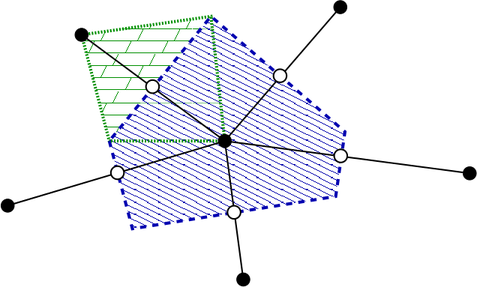
 ), while odd-order unknowns are
associated with edges (open circles, green box
), while odd-order unknowns are
associated with edges (open circles, green box  ).
).
Following the box integration procedure from Sec. 5.1, integration over energy from  to
to
 and over a box
  given on the spatial grid leads to
![∫ H+n ∫
∇x ⋅jl′,m′fl′,m′ − F ⋅Γ l′,m ′fl′,m′dV dH
H−n Bi l,m l,m
∑ ∫ H+n ∫ [
= -1-- Zl,mσ η(x, H ± ℏω η,H)f0,0(x, H ± ℏωη)Z0,0(H ± ℏωη)
Y0,0 η H−n Bi
]
− fl,mZl,m ση(x,H, H ∓ ℏω η)Z0,0(H ∓ ℏω η)dV dH .](diss-et1096x.png) | (5.6) |
The first term on the left hand side is transformed to a surface integral using Gauss’ Theorem,
and then the integrals on the left hand side are decomposed into the individual intersections with
the neighboring adjoint boxes  :
:
![+[ ]
∑ ∫ H n ∫ l′,m′ ∫ l′,m′
− jl,m fl′,m′ ⋅ni,jdA − F ⋅Γl,m fl′,m ′dV dH
Bi,j of Bi H n ∂Bi∩Bi,j Bi∩Bi,j
1 ∑ ∫ H+n∫ [
= ---- Zl,mσ η(x, H ± ℏωη,H )f0,0(x,H ± ℏωη,t)Z0,0(H ± ℏωη)
Y0,0 η H −n Bi
]
− fl,mZl,m ση(x, H, H ∓ ℏωη)Z0,0(H ∓ ℏωη) dV dH ,](diss-et1098x.png) | (5.7) |
where  denotes the outward pointing unit vector with respect to
  and perpendicular to
the common interface of
and perpendicular to
the common interface of  and
and  . Since for even
  the coupling terms
  and
and  take according to Thm. 1 nonzero values for odd
  only, and the scattering operator
exclusively couples terms of the same order
only, and the scattering operator
exclusively couples terms of the same order  , the discretization (5.5) can directly be
inserted:
, the discretization (5.5) can directly be
inserted:
![∑ [ ∫ H+n ∫ H+n ]
βi,n;l′,m ′ Ai,jni,j ⋅ jl′,m′dH − Vi,jF|B ⋅ Γ l′,m′dH
Bi,j of Bi H −n l,m i,j H−n l,m
∫ +
--1-∑ Hn [
= Y0,0 H− Zl,mσ η(x, H ± ℏω η,H )αi,n±n ′η;0,0Z0,0(H ± ℏωη)
η n ]
− αi,n;l,mZl,m ση(x,H, H ∓ ℏω η)Z0,0(H ∓ ℏω η)VidH ,](diss-et1108x.png) | (5.8) |
where  ,
,  as well as the scattering rates are assumed to be homogeneous over the
device, the force
as well as the scattering rates are assumed to be homogeneous over the
device, the force  is approximated by a constant vector
  on
on  and where
  refers to
a suitable index shift such that
refers to
a suitable index shift such that  . Typically, discrete energies are chosen as
fractions of
. Typically, discrete energies are chosen as
fractions of  such that
  is again a discrete energy. It is noteworthy
that the approximation of the force term by a constant vector over
is again a discrete energy. It is noteworthy
that the approximation of the force term by a constant vector over  is mostly
a matter of convenience. One may also use more accurate representations, but the
price to pay is increased computational effort for the evaluation of the integral over
is mostly
a matter of convenience. One may also use more accurate representations, but the
price to pay is increased computational effort for the evaluation of the integral over
 . A dimensional splitting has been used by Hong et al. [42], which can be seen
in this context as considering only the projection
. A dimensional splitting has been used by Hong et al. [42], which can be seen
in this context as considering only the projection  for the integration over
 .
.
A slight rearrangement for better exposition of the unknowns  and
and  yields
![[ ∫ + ∫ + ]
∑ Hn l′,m ′ Hn l′,m ′
βj,k;l′,m′ Ai,jni,j ⋅ H−n jl,m dH − Vi,jF i,j ⋅ H −n Γ l,m dH
Bi,j of Bi
Vi ∑ ∫ H+n
= αi,n±n′η;0,0---- − ση(x,H ± ℏωη,H )Zl,mdH
Y0,0 η H n
V ∑ ∫ H+n
− αi,n;l,m --i- σ η(x, H,H ∓ ℏωη)Z0,0(H ∓ ℏωη)dH .
Y0,0 η H −n](diss-et1124x.png) | (5.9) |
In the case of spherical energy bands, the integrals on the left hand side can be rewritten using (4.2) and (4.3) as
 and
and
 .
.
The discretization of the odd-order projected equations (2.35) is carried out using essentially the
same steps as for the even-order equations, but differs in a few technical details. Integration over
the energy interval from  to
to  and over an adjoint box
  overlapping the boxes
  and
and  leads to
![∫ H+ ∫
n jl′,m′⋅∇ f ′ ′ + F ⋅Γˆl′,m ′f ′ ′dV dH
H−n Bi,j l,m x l,m l,m l,m
∫ H+ ∫ [
= -1--∑ n Z σ (x,H ± ℏω ,H )f (x, H ± ℏω )Z (H ± ℏω )
Y0,0 η H−n Bi,j l,m η η 0,0 η 0,0 η
]
− fl,mZl,m ση(x,H, H ∓ ℏω η)Z0,0(H ∓ ℏω η)dV dH .](diss-et1133x.png) | (5.12) |
Assuming  to be piecewise constant in each of the adjoint boxes
  , application of
Gauss’ Theorem to the first term, and splitting the second integral into the two overlaps with
, application of
Gauss’ Theorem to the first term, and splitting the second integral into the two overlaps with  and
and  leads to
![∫ H+n [∫ ′ ′ ∫ ′ ′
jll,,mm fl′,m′ ⋅ndA + jll,m,m fl′,m ′ ⋅ndA ,
H−n ∂Bi,j∩Bi ∂Bi,j∩Bj
∫ ′ ′ ∫ ′ ′ ]
+ F ⋅ ˆΓ ll,m,m fl′,m ′dV + F ⋅ ˆΓ ll,,mm fl′,m ′dV dH
Bi,j∩Bi Bi,j∩Bj
∑ ∫ H+n ∫ [
= --1- Zl,m ση(x,H ± ℏωη,H )f0,0(x,H ± ℏ ωη)Z0,0(H ± ℏ ωη)
Y0,0 η H−n Bi,j
]
− fl,mZl,mση(x,H, H ∓ ℏωη)Z0,0(H ∓ ℏωη) dV dH .](diss-et1138x.png) | (5.13) |
For odd  , the terms
  and
and  are nonzero for even
  only. Inserting the
expansion (5.4) on the left hand side and (5.5) on the right hand side, one arrives
at
only. Inserting the
expansion (5.4) on the left hand side and (5.5) on the right hand side, one arrives
at
![[ ]
∫ H+n ∫ l′,m ′ ∫ l′,m ′
αi,n;l′,m′ − jl,m ⋅ndA + F ⋅ ˆΓ l,m dV dH
Hn ∂Bi,j∩B[i Bi,j∩Bi ]
∫ H+n ∫ l′,m ′ ∫ l′,m ′
+ αj,n;l′,m ′ − jl,m ⋅ndA + F ⋅Γˆl,m dV dH
Hn ∂Bi,j∩Bj Bi,j∩Bj
2Vi,j ∑ ∫ H+n
= βi,n±n ′η;0,0----- Zl,mση(x, H ± ℏωη,H )Z0,0(H ± ℏωη)dH
Y0,0 η H −n
∑ ∫ H+n
− βi,n;l,m2Vi,j Zl,mσ η(x, H,H ∓ ℏωη)Z0,0(H ∓ ℏωη)dH ,
Y0,0 η H−n](diss-et1143x.png) | (5.14) |
where the scattering rates and the density of states are assumed to be independent of the spatial
variable. Since the current density expansion terms  are also assumed to be constant within
the box
are also assumed to be constant within
the box  , an application of Gauss’ Theorem shows
 | (5.15) |
which allows to replace the integration over the boundary of  by two integrations over the
interface of the boxes
by two integrations over the
interface of the boxes  and
and  . This leads with constant force approximations
  over the
box
over the
box  to
to
![∫ H+n [ l′,m′ l′,m′]
αi,n;l′,m ′ − Ai,jjl,m ⋅nj,i + Vi,jF i,j ⋅ ˆΓ l,m dH
Hn ∫ +
H n [ l′,m ′ ˆ l′,m′]
+ αj,n;l′,m′ − Ai,jjl,m ⋅ni,j + Vi,jF i,j ⋅Γ l,m dH
Hn ∫ +
2Vi,j∑ Hn
= βi,n±n′η;0,0Y0,0 H−n ση(x,H ± ℏωη,H )Zl,mdH
η +
2Vi,j ∑ ∫ Hn
− βi,n;l,m Y---- − ση(x,H, H ∓ ℏωη)Z0,0(H ∓ ℏωη)dH .
0,0 η Hn](diss-et1152x.png) | (5.16) |
The integrals over the coupling coefficients can again be further simplified as in (5.10) and (5.11).
A comparison of the number of vertices required for a MOSFET and for a FinFET
using structured and unstructured grids is given in the following. A comparison for a
one-dimensional  -diode is omitted since there the structured and unstructured meshes
coincide.
-diode is omitted since there the structured and unstructured meshes
coincide.
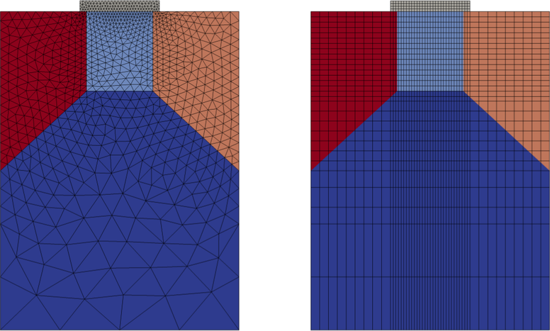
The schematic MOSFET layout shown in Fig. 5.7 consists of  nodes. A much more
aggressive coarsening could have been applied to the left and the right of the device, as well as deep
inside the bulk of the device (bottom). Nevertheless, the structured grid shown at the right, which
has the same grid spacing as the triangular mesh in the channel region, consists of
nodes. A much more
aggressive coarsening could have been applied to the left and the right of the device, as well as deep
inside the bulk of the device (bottom). Nevertheless, the structured grid shown at the right, which
has the same grid spacing as the triangular mesh in the channel region, consists of  nodes,
which consequently leads to about
nodes,
which consequently leads to about  percent more unknowns. Note that the high resolution
inside the channel induces an increased solution deep in the substrate, because so-called hanging
nodes1
are prohibited for the box integration scheme. Therefore, a lower resolution, which would be
typically sufficient deep in the substrate, cannot be obtained there. For demonstration purposes,
only a coarse mesh has been chosen at the contacts. A finer grid at the contacts would result
again in additional grid nodes in the bulk for the structured grid.
percent more unknowns. Note that the high resolution
inside the channel induces an increased solution deep in the substrate, because so-called hanging
nodes1
are prohibited for the box integration scheme. Therefore, a lower resolution, which would be
typically sufficient deep in the substrate, cannot be obtained there. For demonstration purposes,
only a coarse mesh has been chosen at the contacts. A finer grid at the contacts would result
again in additional grid nodes in the bulk for the structured grid.
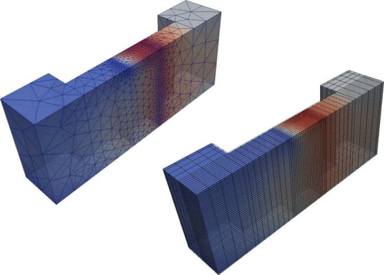
For a fully three-dimensional layout such as that of a FinFET, the difference in the
number of grid points between structured and unstructured grids becomes much larger.
Since the current flow is predominantly near the surface of the fin, a coarser mesh can
be chosen in the center of the fin when using unstructured grids. At the transition
from the source to the channel and particularly from the channel to the drain, a fine
resolution is necessary in order to account for the high electric fields and the heated
carriers in the latter case. The sample meshes of a FinFET depicted in Fig. 5.8 show
that with only  nodes a fine mesh can be obtained in the channel and towards
the drain region, while a structured grid with comparable resolution in the channel
leads to
nodes a fine mesh can be obtained in the channel and towards
the drain region, while a structured grid with comparable resolution in the channel
leads to  nodes, hence the difference is a factor of six. This difference mostly
stems from the spurious high resolution of the structured grid in the source and drain
regions.
nodes, hence the difference is a factor of six. This difference mostly
stems from the spurious high resolution of the structured grid in the source and drain
regions.
 points,
the structured grid leads to
points,
the structured grid leads to  grid points.
 points,
the structured grid is made up of
points,
the structured grid is made up of  points, thus leading to considerably higher
computational costs. For simplicity, only a course mesh has been chosen around the contacts.
points, thus leading to considerably higher
computational costs. For simplicity, only a course mesh has been chosen around the contacts.