Appendix A
Resolvent for Integral Equations
While the computation of integrals in itself is a worthy application of Monte Carlo theory, especially in
the case of high dimensionality of the integration domain, it can be employed to obtain solutions, or at
least estimates, to integral equations.
Recalling that Fredholm integral equations of the second kind
 have a
solution of the form
have a
solution of the form
 as
outlined in Section 4.9. This resolvent series includes repeated integrals which are accessible to Monte
Carlo integration methods.
as
outlined in Section 4.9. This resolvent series includes repeated integrals which are accessible to Monte
Carlo integration methods.
Beginning with examining the integrals in the resolvent series and rewriting them as expectation values
gives
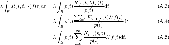 Examining the terms in order of increasing summation index shows
 Recalling Equation 4.184 gives
 where further integrals appear, when expanding
 which can again be evaluated in a similar fashion as an expectation value (Definition 101) with a
random variable (Definition 98).
which can again be evaluated in a similar fashion as an expectation value (Definition 101) with a
random variable (Definition 98).
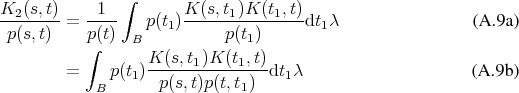
The recursion relation A.7 allows to reuse the obtained result in the subsequent terms and further
recursion reveals that the term for  evaluated using Monte Carlo methods (see Section 6.6.2)
takes the shape
evaluated using Monte Carlo methods (see Section 6.6.2)
takes the shape
 Thus
every term in the series requires an additional random number to be generated in order to calculate an
expectation value. The notion of the procedure is depicted in Figure A.1.
Thus
every term in the series requires an additional random number to be generated in order to calculate an
expectation value. The notion of the procedure is depicted in Figure A.1.