Fundamental physical mechanisms in deposition and etching processes generate both desired and undesired topographic features. In this chapter we provide a basis for understanding and modeling these effects on topography. A common framework for modeling etching and deposition is given, including the terminology used for describing the various physical phenomena and effects.
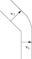
The starting point for both is the nature of flux which arrives from a source above the wafer. The second commonality is how the self-shadowing of an existing profile affects the visibility of the source and how the re-emission from the profile or radiosity affects other points of the profile. The third common aspect is that mechanical and chemical reactions at the surface determine the local advancement rate and are one of the most challenging aspects of deposition and etching. The final common characteristic of deposition and etching is the time-advance of the surface profile. In this chapter we focus on this final common aspect.
![\includegraphics[width=0.5\linewidth]{protective2}](img113.png)
|
The local fluxes and etch or deposition reactions provide sufficient information on how the surface is to be deformed for a short time step. The time evolution of the profile requires many time increments which allow the change of the profile shape to influence its future shape through shadowing, etc. As the surface evolves there may be major topological changes. For example, outgrows of the material from sides of a trench might collide and close off a void, or etch fronts from two trenches might move laterally, collide and form a tunnel or an air bridge.
To ease the presentation a simpler two-dimensional case will
be used. In two dimensions the profile is sometimes said to be made of
line segments and intersections points which may also be called
nodes. Figure 3.3 shows the simulation result of an
isotropic deposition of a material into a rectangular structure. It
can be seen easily that the boundary is expanded radially outward for a time step
![]() . The top right convex outward corner point causes a fan
(cf. Figure 3.3) of facets to be generated which creates a rounded section in the profile at
time
. The top right convex outward corner point causes a fan
(cf. Figure 3.3) of facets to be generated which creates a rounded section in the profile at
time ![]() . At the concave outward corner the planar fronts from the
horizontal and vertical facets intersect in a line which is
the location of a new corner point. These collisions where
overlapping fronts occur and some information about the initial
profile is lost are said to be shocks (cf. Figure 3.3). Note that shocks and fans
play a very important role in determining the changes of topography
during processing. For isotropic etching the profile moves from the
surface into the material as shown in
Figure 3.4. As expected the convex outward corner
now produces a shock and the concave corner point produces a fan.
. At the concave outward corner the planar fronts from the
horizontal and vertical facets intersect in a line which is
the location of a new corner point. These collisions where
overlapping fronts occur and some information about the initial
profile is lost are said to be shocks (cf. Figure 3.3). Note that shocks and fans
play a very important role in determining the changes of topography
during processing. For isotropic etching the profile moves from the
surface into the material as shown in
Figure 3.4. As expected the convex outward corner
now produces a shock and the concave corner point produces a fan.
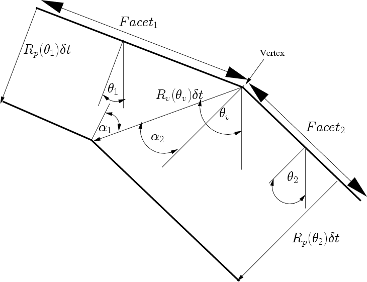 |
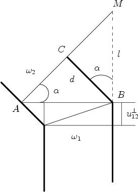
To understand faceting of the initial profile the advancement
of two neighboring facets as shown in
Figure 3.5 is considered. The direction and rate of
advance of a vertex where two facets intersect is of key interest. The two
facets have downward
normals which form angles
![]() and
and
![]() with respect
to the vertical downward direction. They advance a distance which is
the product of the planar etch rate for their orientation
with respect
to the vertical downward direction. They advance a distance which is
the product of the planar etch rate for their orientation
![]() and time step
and time step ![]() as
as
![]() and
and
![]() , respectively. The vertex moves at an angle
, respectively. The vertex moves at an angle
![]() and a rate
and a rate
![]() and therefore a distance
and therefore a distance
![]() . The angles of the path of this vertex with respect to the normal of the
two facets are
. The angles of the path of this vertex with respect to the normal of the
two facets are
![]() and
and
![]() which are
which are
![]() and
and
![]() ,
respectively. Projecting the distance of movement of this
vertex onto the distances advanced by the facets gives the two following
equations:
,
respectively. Projecting the distance of movement of this
vertex onto the distances advanced by the facets gives the two following
equations:
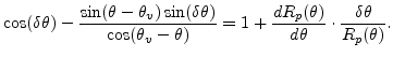
Taking the ratio between (3.1) and (3.2) and
eliminating
![]() gives
gives
Once
![]() is known the associated rate
is known the associated rate
![]() can
be found from (3.1) and (3.2) and is of course higher
than
can
be found from (3.1) and (3.2) and is of course higher
than
![]() and
and
![]() .
.
(3.3) makes a number of interesting predictions about
the physical nature of the motion of the vertex. Assuming
that
![]() and
and ![]() is not a
function of the facet angle
is not a
function of the facet angle ![]() , then the right hand side of
(3.3) is unity, forcing
, then the right hand side of
(3.3) is unity, forcing
![]() or
or
![]() which means that the
intersection vertex moves along the bisecting angle.
which means that the
intersection vertex moves along the bisecting angle.
Another important case is that ![]() increases with the angle
increases with the angle
![]() . This makes the right hand side of (3.3)
. This makes the right hand side of (3.3)![]() which leads to
which leads to
![]() or
or
![]() . This means that the
faster moving facet will encroach into the region of the slower moving
facet and likely expands in size.
. This means that the
faster moving facet will encroach into the region of the slower moving
facet and likely expands in size.
To further explore how the movement of a facet depends on the shape of
the rate function, the direction of travel of a facet at angle ![]() with rate function
with rate function
![]() is now derived in a limiting
case. Assuming that the angle between a facet pair is small enough,
their intersection vertex will propagate in the direction of motion of
the facet. This limiting case can be determined from
(3.3) by taking the special case of
is now derived in a limiting
case. Assuming that the angle between a facet pair is small enough,
their intersection vertex will propagate in the direction of motion of
the facet. This limiting case can be determined from
(3.3) by taking the special case of
![]() and
and
![]() and letting
and letting
![]() go to
zero. Substituting
go to
zero. Substituting
![]() and
and
![]() in
(3.3) and expanding
in
(3.3) and expanding ![]() in a Taylor series gives
in a Taylor series gives
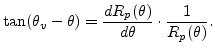
Letting
![]() go to zero in (3.4) gives
go to zero in (3.4) gives
(3.5) indicates that a facet at angle ![]() moves
laterally with a rate component proportional to the slope of the rate
function
moves
laterally with a rate component proportional to the slope of the rate
function
![]() as well as
normal to the surface at the usual rate
as well as
normal to the surface at the usual rate
![]() .
.
Regarding the evolution of facets each facet has a plane associated with it. The plane moves with a given normal speed which may be different for different facets. The boundaries of the facets are determined by the intersection of the planes. The two-dimensional evolution near a corner is shown in Figure 3.6. If we use a level-set method where the normal speed is a simple interpolation between the two normal speeds, then the corners would be rounded, as shown in Figure 3.7 (in particular, an arc of a circle would arise, if the two speeds are the same). In order to keep flat facets and sharp corners, the following precautions must be made. The evolution of a smooth curve only depends on the normal speed, the addition of a tangential component only has the effect of changing the parameterization of the curve. With a velocity that has a proper tangential component to the facet and is directed towards a corner, the facets will evolve maintaining sharp
 |
In order to minimize the corner rounding during the movement of a
boundary the approach introduced by Russo and Smereka [71] can
be used where the speed of each facet must be specified.
Consider an interface consisting of ![]() facets, with normals
facets, with normals
![]() and absolute value of normal
speeds
and absolute value of normal
speeds
![]() for
for ![]() . Let
. Let
![]() be the normal
at a given point of the interface.
be the normal
at a given point of the interface.
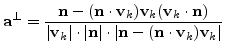
In order to compute the proper velocity of the surface at a given
point, first the facet is selected which is closest in direction to
![]() , i.e., for which
, i.e., for which
![]() is a maximum,
is a maximum,
| (3.6) |
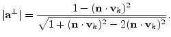
Next the following velocity is defined
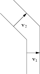
Some simple geometric considerations as shown in Figure 3.8 and the following equations help us to find the tangential speed that must be added to keep a sharp corner.
| (3.10) |
| (3.11) |
The quantity ![]() can then be chosen equal to
can then be chosen equal to ![]() , where
, where
| (3.12) |
For a faceted interface
![]() , because
, because
![]() and the facet
will evolve with the standard normal speed. On the other hand, if we
evolve the whole interface with the velocity
and the facet
will evolve with the standard normal speed. On the other hand, if we
evolve the whole interface with the velocity
![]() , then the
corners get rounded as shown in Figure 3.7. When the corners
become slightly rounded, then
, then the
corners get rounded as shown in Figure 3.7. When the corners
become slightly rounded, then
![]() becomes directed towards the corners
and the surface will move with a velocity that will try to keep the
corners sharp.
becomes directed towards the corners
and the surface will move with a velocity that will try to keep the
corners sharp.
Choosing a small value for
![]() , the vector
, the vector
![]() is basically a
unit vector whenever
is basically a
unit vector whenever
![]() is not aligned with the facets. Neglecting
is not aligned with the facets. Neglecting
![]() , the normal speed
, the normal speed
![]() can be calculated from
(3.7) with the following equation
can be calculated from
(3.7) with the following equation
 |
(3.14) |
Substituting (3.15) in (3.13) gives the normal speed of our model for the level set function
| (3.16) |
In Chapter 7 we will present the application of this method to get the trenches with a minimal corner rounding during the simulation of an etching process.
![\includegraphics[width=0.5\linewidth]{shadowing}](img112.png)
![\includegraphics[width=0.8\linewidth]{figures/faceting-deposition2}](img116.png)
![\includegraphics[width=0.8\linewidth]{figures/faceting-etching}](img117.png)
![$\displaystyle \mathbf{a}=\frac{\mathbf{n}-(\mathbf{n}\cdot\mathbf{v}_{k})\mathb...
...{n}\cdot\mathbf{v}_{k})\mathbf{v}_{k}\vert^{2}+\varepsilon ^{2}]^{\frac{1}{2}}}$](img165.png)