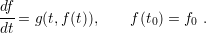
Time dependence analysis is not particularly interesting for elastic deformations, since the material recovers entirely after load removal. However, for plastic deformations, the duration of a force application defines the amount of permanent deformation within the body. Actually, plasticity has an elegant treatment with the FEM, which has been developed along the years [40]. Although plastic deformation is studied in this work, the classical approach of plasticity is not used. Instead, a specific model based on ordinary differential equations (ODE) is employed as will be discussed in Chapter 5. This section intends to provide the background for the treatment of these kinds of equations. Time dependent problems can be presented in the general form by [63]
|
| (3.37) |
These types of equations, where the solution to the first step ( ) is
known, are defined as initial value problems (IVP). High order ODEs can always be
converted to a system of N first order equations in the same form as (3.37) by
substitution. For example, the ODE
) is
known, are defined as initial value problems (IVP). High order ODEs can always be
converted to a system of N first order equations in the same form as (3.37) by
substitution. For example, the ODE  can be rewritten as
  and
and
 .
.
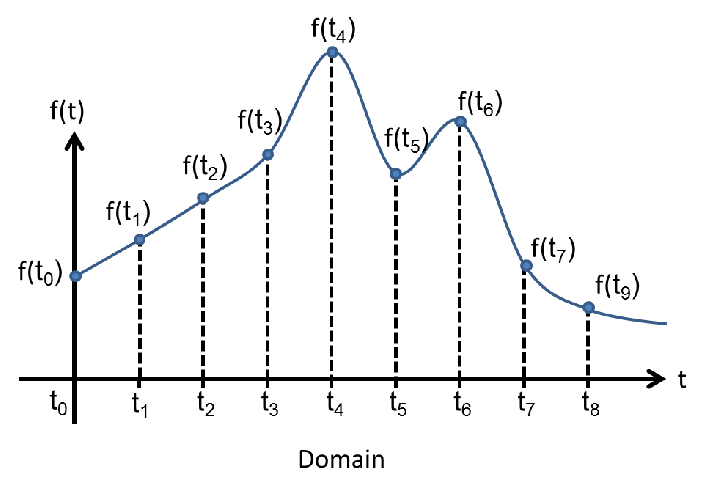
In general, the strategy for solving (3.37) numerically consists of the division of the domain into small time steps; and for each step the solution is computed as shown in Fig. 3.9.
Numerical methods for ODEs can be divided between explicit and implicit methods. The
former handles (3.37) by computing the next state of the system based solely on the current
state ( ), while implicit methods require also the future state
(
), while implicit methods require also the future state
( ). The formulation of implicit methods seems
rather paradoxical, but in practice only an estimation of the future state is used to
compute
). The formulation of implicit methods seems
rather paradoxical, but in practice only an estimation of the future state is used to
compute  . Explicit methods are more intuitive and easy to implement, but they
require an unreasonable number of steps to properly approximate problems with
fast variations, the so called stiff problems, for which implicit methods are more
suitable.
. Explicit methods are more intuitive and easy to implement, but they
require an unreasonable number of steps to properly approximate problems with
fast variations, the so called stiff problems, for which implicit methods are more
suitable.
In order to exemplify both categories, consider the approximations for the derivatives
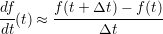 | (3.38) |
and
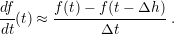 | (3.39) |
Substituting (3.38) and (3.39) in (3.37) the relations hold
 | (3.40) |
 | (3.41) |
One can notice the particular difference between the representation of (3.40) and (3.41). For
the first case the unknown variable ( ) is defined explicitly by the terms on the
right hand side. In the second case the unknown (
) is defined explicitly by the terms on the
right hand side. In the second case the unknown ( ) is needed in order to compute the
function
) is needed in order to compute the
function  , which leads to an implicit definition of
  . Each equation defines a method
for the solution of (3.37), where (3.40) is known as the Euler method and (3.41) as backward
Euler method.
. Each equation defines a method
for the solution of (3.37), where (3.40) is known as the Euler method and (3.41) as backward
Euler method.
In the scope of this work, implicit methods are more relevant, mainly because of
exponential variations in the models for describing plasticity in Chapter 5. The so called
Back Differentiation Formula (BDF) is the employed method for ODEs. The BDF
method approximates the function  by a Lagrangian polynomial as defined by
[64]
by a Lagrangian polynomial as defined by
[64]
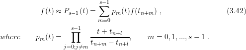
The meaning of  will become clear soon, but right now
  can be understood as the
degree of the Lagrange polynomial. From the polynomial definition (3.42) the BDF method
can be built. The derivative of
can be understood as the
degree of the Lagrange polynomial. From the polynomial definition (3.42) the BDF method
can be built. The derivative of  is approximated by the derivative of the Lagrangian
polynomial as described by
is approximated by the derivative of the Lagrangian
polynomial as described by
 | (3.43) |
From (3.43) one can see that  defines the number of past states, which is used to calculate
the current state of the system. As
defines the number of past states, which is used to calculate
the current state of the system. As  increases the local error of the method reduces, but
for
increases the local error of the method reduces, but
for  the BDF is no longer convergent. Naturally, higher values of
  imply higher
computational demands; hence a compromise between speed and accuracy must be met.
Table 3.1 represents the BDF method after expansion of the Lagrangian polynomial for
imply higher
computational demands; hence a compromise between speed and accuracy must be met.
Table 3.1 represents the BDF method after expansion of the Lagrangian polynomial for
 .
.
| Table 3.1.: | Expansion of the Lagrangian polynomial for  . . |
| Order | Expression | |||
| BDF 1 |  |
|||
| BDF 2 |  |
|||
| BDF 3 |  |
|||
| BDF 4 |  |
|||
| BDF 5 |  |
|||
In practice, the computation for each time step requires the solution of a non-linear
equation. Newton’s method is the most common choice for solving the non-linear problem,
but other methods can be more suitable, depending on the form of  . As an initial guess,
an explicit method (such as the Euler method) can be used to provide a reasonable choice
for
. As an initial guess,
an explicit method (such as the Euler method) can be used to provide a reasonable choice
for  .
.
Naturally, the effort to compute the solution at each time step is bigger for BDF methods
than for explicit methods, but the argument for their utilization lies on the stability.
Implicit methods are more stable than explicit methods, an important feature for the
numerical solution of stiff ODEs. Such problems are by definition numerically unstable,
which means that small deviations of the solution in a particular step lead to a large error in
the subsequent steps. In fact, it can be proved that for  , the BDF is A-stable [64].
This means that for an ODE in the form
, the BDF is A-stable [64].
This means that for an ODE in the form  , the exact solution (
 ) and the
BDF solution are asymptotically equivalent for
) and the
BDF solution are asymptotically equivalent for  . Such a condition is only valid in the
Euler method for very small time steps [64]. Evidently,
. Such a condition is only valid in the
Euler method for very small time steps [64]. Evidently,  is not a general case, but it
is commonly used as a test problem to evaluate the stability of numerical methods for
ODEs.
is not a general case, but it
is commonly used as a test problem to evaluate the stability of numerical methods for
ODEs.