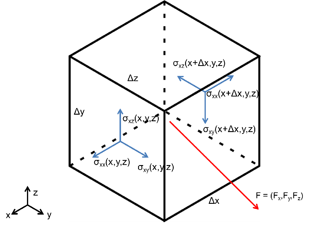
| Figure 3.7.: | Inifinitesimally small stress cube. The stress is defined in the face of the
cube, however only  is explicitly shown. The others are omitted for the sake of
clarity in the picture. is explicitly shown. The others are omitted for the sake of
clarity in the picture. |
Static equilibrium is the most common situation for mechanical problems in semiconductor devices. In equilibrium, the sum of forces (and momentum) in a body must be zero, including those produced by stress. In order to derive the equilibrium equations consider an infinitesimally small solid and the stress distribution on its faces, as depicted in Fig. 3.7.
| Figure 3.7.: | Inifinitesimally small stress cube. The stress is defined in the face of the
cube, however only is explicitly shown. The others are omitted for the sake of
clarity in the picture. |
Each stress component is assumed to be a continuous differentiable function of x, y, and z. Hence, they can be expanded by Taylor series and the stress on the faces of the infinitesimal cube can be arranged as
 | (3.25) |
 | (3.26) |
 | (3.27) |
The body can be under the influence of an external disturbance (e.g. gravity), which must be considered in the equilibrium equations. In Fig. 3.7 the sum of all external forces is represented by the vector F. The equilibrium of forces in the x-direction can be obtained by
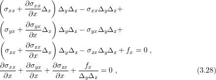
where  is an external force in the x-direction. A similar treatment can be applied in the
y-direction and the z-direction. Thus, the equilibrium equations can be summarized
by
is an external force in the x-direction. A similar treatment can be applied in the
y-direction and the z-direction. Thus, the equilibrium equations can be summarized
by
 | (3.29) |
where  ,
,  and
and  are the external forces per unit area in the corresponding
Cartesian direction.
are the external forces per unit area in the corresponding
Cartesian direction.
A great deal of mechanical analysis in microelectronics relies on the elastic theory. However, solving its fundamental equation is challenging. The solution is usually unknown for varying geometries and conditions faced by the engineering design. The few known solutions are only available to simple geometries (e.g. circle, square) and restricted conditions, which can lead to an oversimplification of the analysis. In order to enhance the mechanical analysis, FEM can be used to compute the elastic equations on general geometries and conditions. It provides means to simulate elastic problems by discretizing its fundamental equations.
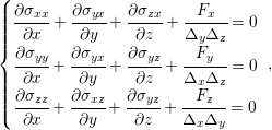
To a generalized treatment of elastic problem by FEM, consider the problem depicted in
Fig. 3.8. The presented problem is rather general concerning geometry and conditions.
Dirichlet and Neumann boundary conditions are presented ( on
on  and
and  on
on  , respectively). Additionally, the shape is amorphous, meaning no preferred
geometry.
, respectively). Additionally, the shape is amorphous, meaning no preferred
geometry.
| Figure 3.8.: | General elastic problem. B is the body force and g an external load. The
surface  is free to move, while is free to move, while  is constrained. is constrained. |
Within this section, a tensorial treatment will be used for the sake of notation simplicity. A table with tensorial definitions, properties and operations is available in the appendix.
The body is assumed to be in static equilibrium; therefore (3.29) must be satisfied. The system (3.29) can be rewritten in its tensorial form for convenience together with its boundary conditions by

Following the same procedure to derive the FEM in the last session, (3.30) is multiplied by a
function  . However, this time
 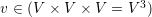 is a vectorial function. Since the
static equilibrium problem is three-dimensional, a test function is needed for each
dimension. The multiplication result is described by
is a vectorial function. Since the
static equilibrium problem is three-dimensional, a test function is needed for each
dimension. The multiplication result is described by
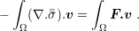 | (3.31) |
The next step is the simplification of (3.31). In the last section the integration by parts was used. For the current case, the first Green identity as described in [62] is applied
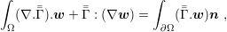 | (3.32) |
where  is a second order tensor and
  is a vector. An intriguing fact is that (3.32) is the
equivalent of the integral by parts in higher dimensions. Proceeding with the proper
substitution of (3.32) in (3.31) and some rearrangement, (3.31) can be rewritten
as
is a vector. An intriguing fact is that (3.32) is the
equivalent of the integral by parts in higher dimensions. Proceeding with the proper
substitution of (3.32) in (3.31) and some rearrangement, (3.31) can be rewritten
as
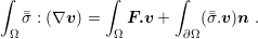 | (3.33) |
So far, the equilibrium equations were stated in terms of the stress tensor, but the real unknown is the displacement. As seen previously (Section 2.2.1) stress and strain can be derived from displacement but the opposite is not as straightforward. Furthermore, the description by means of stress challenges the imposition of boundary conditions on the displacement field. Hence, a tensorial description of stress and strain is considered using
![[ E ν ] ¯ E
¯¯σ = (1-+-ν)(1−-2ν)∇.u ¯I + 1+-νϵ¯¯(u )](diss355x.png) | (3.34) |
and
![¯¯ϵ = 1-[(∇u )T + ∇u ] ,
2](diss356x.png) | (3.35) |
respectively. Consistently, the definitions (3.34) and (3.35) are equivalent to (2.22) and (2.10), but in Section 2.2.1 the physical meaning of the equations was preferred over simplicity.
Finally, substituting (3.34) and (3.35) in (3.33) the variational formulation of (3.30) is obtained as
![Find u ∈ (V3) such that ∀v ∈ (V3)
∫ [ ] ∫ ∫
-----E-ν-----(∇.u )(∇.v) + G-[(∇u )T + ∇u ] : ∇v = F.v + g.v .
Ω (1 + ν)(1− 2ν ) 2 Ω ∂Ω
(3.36)](diss357x.png)
From this point the same development of the previous section can be implemented.
Therefore, the coordinate space  is dicretized (a basis set for each dimension), the basis
functions are chosen following the pre-established criteria and the linear system is built.
Recall the previous discussion regarding 2D and 3D problems, which fit to this
analysis.
is dicretized (a basis set for each dimension), the basis
functions are chosen following the pre-established criteria and the linear system is built.
Recall the previous discussion regarding 2D and 3D problems, which fit to this
analysis.
For this specific problem, those aspects will not be discussed here, but they are available in several textbooks about the FEM in mechanical problems [57]. Furthermore, they are not essentially different from the 1D problem presented in the previous section. The dimensional generality of FEM is an asset of the technique.