 is endowed with inner products for real functions defined
by
is endowed with inner products for real functions defined
by
The manner in which the FEM was presented in this work makes the geometrical
interpretation of the method a natural consequence. In this section it will be shown that this
concept is intimately connected to the error of the linear space discretization of the FEM.
In order to proceed smoothly through the upcoming discussion, consider that
the linear space is endowed with inner products for real functions defined
by
 | (3.19) |
Furthermore, consider the norm induced by the inner product (3.19) as
 | (3.20) |
Consequently, the variational form (3.5) and the discrete variational form (3.10) can be rewritten as
 | (3.21) |
and
 | (3.22) |
The discrete problem solution ( ) is computed by FEM as seen in the previous sections,
but the exact solution of the BVP problem is given by solving the continuous variational
form. Therefore, it is natural to ask how distant
) is computed by FEM as seen in the previous sections,
but the exact solution of the BVP problem is given by solving the continuous variational
form. Therefore, it is natural to ask how distant  is from
  . The answer of this question
leads to a geometrical view of the FEM.
. The answer of this question
leads to a geometrical view of the FEM.
Consider  . The function
  also belongs to
  since
since  . Therefore, for every
 (3.22) can be subtracted from (3.21), given by
 | (3.23) |
As an inner product, (3.19) must hold the orthogonality property (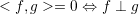 ).
This means that the discretization error (
).
This means that the discretization error ( ) is orthogonal to the space
  . As a
consequence, the solution
. As a
consequence, the solution  is the orthogonal projection of the exact solution
  in
in  .
Fig. 3.6 illustrates this principle.
.
Fig. 3.6 illustrates this principle.
| Figure 3.6.: | Geometrical interpretation of Galerkin’s method. The solution ( ) of
the original problem is projected ( ) of
the original problem is projected ( ) in the space defined by the basis of ) in the space defined by the basis of  .
Galerkin’s method can be understood as the procedure to find this projection. .
Galerkin’s method can be understood as the procedure to find this projection. |
As a result of the orthogonal projection, the element  is the closest function to
  in
comparison to all elements of
in
comparison to all elements of  . Hence, the error of discretization is bounded according to
[56]
. Hence, the error of discretization is bounded according to
[56]
 | (3.24) |
The relation (3.24) will not be proved here, but it is intuitively clear when orthogonal
projections are kept in mind. In conclusion, FEM provides the best approximation
of the exact solution  in the discretized space
  , when the norm (3.20) is
considered.
, when the norm (3.20) is
considered.
At this point, the advantage of the original Galerkin’s imposition for the solution  and
the test function
and
the test function  becomes evident –
  and
and  , respectively, for the discrete
formulation – to reside in the same linear space. The formulation gains some formal support,
especially regarding the discretization error, since it is guaranteed that the FEM solution is
the best choice in a particular space.
, respectively, for the discrete
formulation – to reside in the same linear space. The formulation gains some formal support,
especially regarding the discretization error, since it is guaranteed that the FEM solution is
the best choice in a particular space.