Analytic Solution for the Stress Around One TSV

4.3.2 Analytic Solution for the Stress Around One TSV

A previous work [82] from Lu et al. has developed an analytical solution for the curve sketched in Fig. 4.5 for filled TSVs. Unfortunately, their solution and solving strategy cannot be applied to unfilled vias. The exact solution for such cases will be developed in this section.

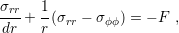
Consider the equilibrium equation (3.29) in cylindrical coordinates as

σrr 1 ---+ --(σrr − σϕϕ) = − F , dr r

(4.1)

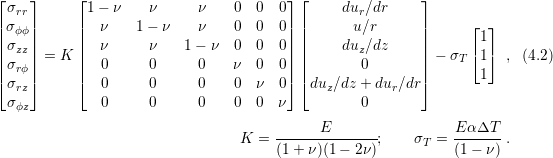
and Hooke’s Law with a thermal expansion (2.24) also adapted for cylindrical coordinates in axis-symmetric geometries as stated in [39]

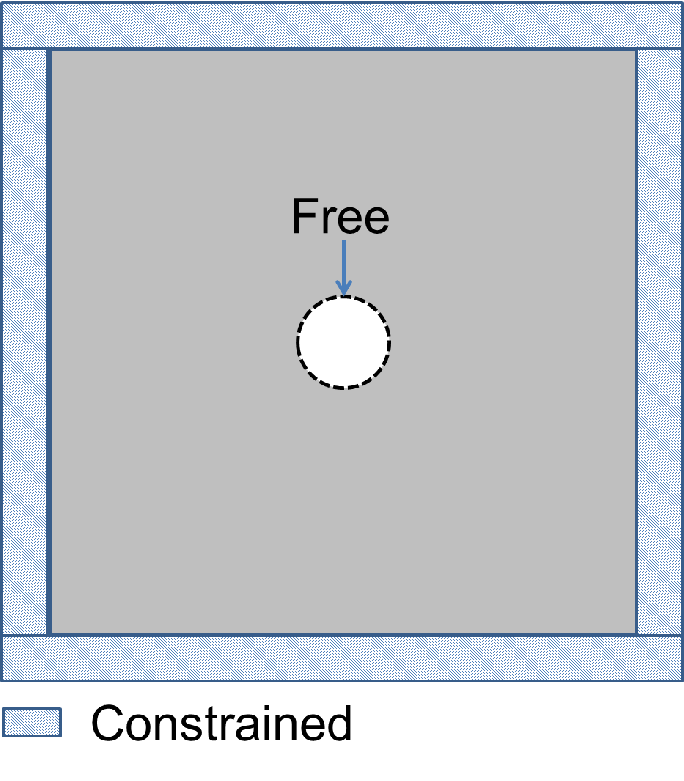
⌊ ⌋ ⌊ ⌋ ⌊ ⌋ σrr 1− ν ν ν 0 0 0 dur∕dr || σϕϕ|| || ν 1− ν ν 0 0 0|| || u∕r || ⌊ 1⌋ || σzz|| || ν ν 1 − ν 0 0 0|| || duz∕dz || ⌈ ⌉ || σrϕ|| = K || 0 0 0 ν 0 0|| || 0 ||− σT 1 , (4.2) ⌈ σrz⌉ ⌈ 0 0 0 0 ν 0⌉ ⌈duz∕dz + dur∕dr ⌉ 1 σ 0 0 0 0 0 ν 0 ϕz ------E------- E-αΔT-- K = (1 + ν)(1− 2 ν); σT = (1− ν ) .

The problem domain is assumed to be a plate of a single material with an unconstrained hole in the middle and constrained borders as depicted in Fig. 4.6.

pict

Figure 4.6.:

Problem description of the stress created by unfilled TSVs due to thermal expansion.

The plane strain approximation is imposed, thus the normal strain in z-direction vanishes and Hooke’s law in (4.2) is simplified as

[ ] [ ][ ] ⌊ 1⌋ σrr 1 − ν ν dur ∕dr ⌈ ⌉ σϕϕ = K ν 1 − ν u∕r − σT 1 . 1

(4.3)

No body force is present in the structure, hence (4.2) becomes a homogeneous PDE with the solution in the displacement field given by

B u(r) = Ar + -- , r

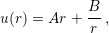(4.4)

where A and B are integration constants. The unfilled via cross section is composed of more materials layers (two oxide layers and one metal layer), therefore Fig. 4.6 does not describe fully the original problem. However, the general solution is still useful. The material properties manifest themselves only in the integration constants. Hence, the solution differs solely by constants among the materials as shown in Fig. 4.7.

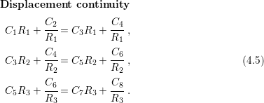
The different constants can be obtained by ensuring stress and displacement continuity in the interfaces and, of course, by applying the boundary conditions of the problem as in (4.5), (4.6), and (4.7).

Displacement continuity C2 C4 C1R1 + R--= C3R1 + R--, 1 1 C3R2 + C4-= C5R2 + C6-, (4.5) R2 R2 C6 C8 C5R3 + ---= C7R3 + ---. R3 R3

Stress continuity [ ] [ ] K C + (2ν-−-1)C2- = K C + (2ν −-1)C4 , oxide 1 R21 W 3 R21 [ ] [ ] (2ν-−-1)C4 (2ν −-1)C6 KW C3 + R22 = Koxide C5 + R22 , (4.6) [ ] [ ] (2-ν −-1)C6 (2ν −-1)C8 Koxide C5 + R2 = KSi C7 + R2 . 3 3

Boundary conditions [ ] σrr(R0 ) = Koxide C1 + (2ν −-1)C2 = 0 , (4.7) R20 u(R4) = C7R4 + C8-= 0 . R4

pict

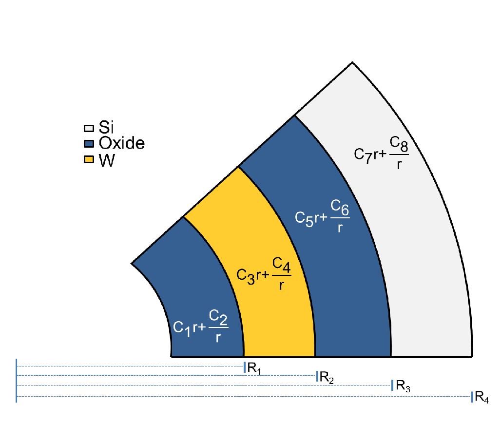
Figure 4.7.:

Solution of the different materials. The solution form is kept, since the equilibrium equation must be satisfied in every material. The constants are solely determined by the material parameters and via geometry. They can be computed by imposing boundary conditions and interface conditions (continuous displacement and radial stress between the interfaces).

Although the full development of the analytical solution is feasible, it is very lengthy. A faster approach is to compute the constants directly with a linear solver or with the transfer matrix method.

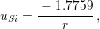
An additional consideration can be included to simplify the solution. Since the domain dimensions are far larger than the stress spread zone, it is possible to consider the exact solution under the infinite plane approximation. In that situation the constant value C7 vanishes and one can calculate the displacement and stress in silicon for the standard unfilled TSV by

−-1.7759- uSi = r ,

(4.8)

[( ) ( )] Si ---ESi(1−-ν-)--- -−-1.7759- --1.7759ESi-νSi-- σrr = (1+ νSi)(1− 2ν ) r2 − r(1 + νSi)(1− 2ν)+ σT , and

(4.9)

[( E ν ) ( − 1.7759) ] 1.7759E (1− ν ) σSϕiϕ = -------SiSi----- ----2---- − -------Si-------+ σT . (1 + νSi)(1 − 2ν) r r(1 + νSi)(1 − 2ν)

(4.10)

In Fig. 4.8 the displacement evolution in silicon along the radius of the TSV is shown in comparison with the exact solution given by (4.8) . One can notice that this approach also allows for the calculation of the exact solution for filled TSVs.

pict

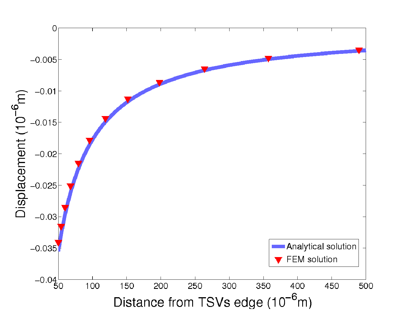
Figure 4.8.:

Comparison between the FEM solution and the analytical solution described in this section.

[next] [prev] [prev-tail] [front] [up]