Subsections

• 6.4.1 Distribution Function Based Estimation
• 6.4.2 Carrier Temperature Based Evaluation
• 6.4.3 Results and Discussion

6.4 Acceleration Integral Estimation in Drift-Diffusion

The long simulation times required for the thorough calculation of the distribution function using the Monte Carlo method make the presented hot-carrier degradation model unsuitable for a wide spread industrial use. To overcome this problem, it is investigated in this work how to estimate the acceleration integral within the drift-diffusion framework. The absence of the distribution function makes only two basic approaches feasible. First, the distribution function can be approximated so that the integrals in equations (6.25) and (6.26) can be evaluated. Or second, a fitting formula for the acceleration integral has to be found. It is expected, that the disadvantages of such estimations, especially the reduced accuracy, can be partly compensated by the enormous performance gain which is achieved by omitting the Monte Carlo simulations. Another positive side effect of the short simulation time is the possibility to evaluate the acceleration integral at each time step. This means that the rate equations can be solved for every stress time step. Therefore self-consistent degradation simulations can be performed.

The two concepts have been implemented and used in MINIMOS-NT. The implementation is based on the formulation in (6.50) and is solved self-consistently in the drift-diffusion framework. The occupation of created interface traps is modeled according to the Shockley-Read-Hall formalism, including the contributions to the Poisson and the continuity equation.

In the following, the simulations are based on the $0.5$ µm device depicted in Fig. 6.5. This device was chosen because it is the only one of the devices analyzed in Section 6.3.2 where the electron contribution is sufficient for the degradation modeling (compare Fig. 6.6). Therefore, the effect of holes can be neglected. This limitation is important, because in the drift-diffusion scheme the carrier energy, and hence, the carrier distribution function can only be evaluated from the electric field. Therefore, in this paradigm it is impossible to distinguish between the individual carrier energies, and hence, to separate trap creation processes. To summarize, the hole contributions would introduce additional obstacles regarding the non-locality of the electric field, impact-ionization, and hole energy which could not be reproduced in the drift-diffusion model as required.

Where applicable, the parameters have been chosen equally to the results which were calibrated within the Monte Carlo approach. The mobility degradation model in (4.13) is used to contribute to the interface charge scattering.

6.4.1 Distribution Function Based Estimation

For the evaluation of the acceleration integral, first an approximation for the distribution function has to be defined. Possibilities for this have been shown in Section 4.3.2. The formulation by Grasser in (4.28) gives the best results and is, therefore, used for the investigations in this work. The parameter $\ensuremath{\mathcal{E}}_\mathrm{ref}$ is always evaluated using (4.29). However, the parameter $b$ was either evaluated using (4.31), or, as has been discussed in Section 4.3.2, is set to $b=3.0.$ Both variants are used in the following. The acceleration integral for electrons is computed using (6.25) and (6.26). The calibrated reference curve based on the Monte Carlo results is calculated using $\ensuremath{\ensuremath{\mathcal{E}}_\mathrm{th}}=0.1$ eV. For the estimations in this section, however, different attempts with different threshold energies have been applied.

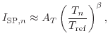
The results are summarized in Fig. 6.9. The reference data clearly show a peak of the acceleration integral at the drain edge of the gate at 1 µm. Both approximations, which use either a constant or non-constant value for $b,$ result in a peak at the very same position. However, a second peak is also pronounced. In some constellations shown, this second peak is even more prominent. It is shifted towards the channel and is visible at the position of approximately 0.9 µm, which is near the pn-junction. This peculiarity can be explained by the interplay between the electric field and the electron concentration along the channel. In this model, both quantities influence the acceleration integral. The electric field explicitly defines the carrier distribution function, while the concentration enters via the normalization condition. Roughly speaking, the acceleration integral behavior can be explained by the product of the electric field and the concentration. Both quantities have extreme values at the end of the gate, whereas the electric field has a maximum and the carrier concentration a minimum. Here is the position of the first maximum. Towards the channel, the electric field decreases and the carrier concentration increase. This combination leads to the second maximum. By comparing the different approaches in Fig. 6.9, one can see that the curve in Fig. 6.9(d) is the only one that suppresses this second peak. This simulation uses the constant exponent $b=3.0$ and a threshold energy of 1.5 eV. Hence, this combination is selected to be used in the following.

Figure 6.9: Evaluation of the acceleration integral for electrons in the $0.5$ µm test device using different representations of the distribution function and different threshold energies in comparison to reference Monte Carlo data ( $\ensuremath {\ensuremath {\mathcal {E}}_\mathrm {th}}=0.1$ eV). The estimations show two peaks, one at the end of the gate, the other near the pn-junction. These two peaks come from an interplay between the electric field and carrier concentration along the channel.

The propagation of the interface trap creation over degradation time can be seen in Fig. 6.10(a). The flat area left to the main peak in the acceleration integral clearly maps to the flattened area in the $N_\mathrm {it}$ profile. The constantly increasing interface trap density in the range from approximately 0.7 to 0.9 µm is caused by the MP process.

Figure 6.10: The evolution of the interface trap concentration with the stress time. The solid lines show the degradation using the distribution function estimation with the acceleration integral from Fig. 6.9(d) (a) and the carrier temperature based estimation (b). The dashed lines are the references from the Monte Carlo based simulations.

(a)

(b)

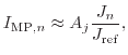
The final degradation of the drain current using this approximation is shown in Fig. 6.11. It can be seen that the overall linear drain current change vs. time within the measurement window can be represented. However, the additional plateau in the peak area of the acceleration integral leads to an additional bending in the drain current degradation curve between 100 and 1000 s.

Figure 6.11: Measured and simulated relative drain current degradations. Simulations are performed using the Monte Carlo, the distribution function (DF) based, and the carrier temperature (CT) based estimation.

6.4.2 Carrier Temperature Based Evaluation

As shown above, the attempt to evaluate the acceleration integral based on artificially created distribution functions does not give satisfying results. Therefore, an empirical approach is proposed, which employs the carrier temperature. The acceleration integral of the SP process is driven by high-energy carriers. It is therefore linked to the electron temperature $T_n$ and the empirical formula is used

$$I_{\ensuremath{\mathrm{SP}},n} \approx A_T \left( \frac{T_n}{T_\mathrm{ref}} \right) ^ \beta ,$$ (6.51)

where $A_T,$ $T_\mathrm{ref},$ and $\beta$ are fitting parameters. The carrier temperature is evaluated employing the energy balance equation in the stationary homogenous case according to Section 4.3.1. For the MP process the electron flux rather than energy is important. As a result, the electron current density $J_n$ enters the expression for the acceleration integral of the MP process

$$I_{\ensuremath{\mathrm{MP}},n} \approx A_j \frac{J_n}{J_\mathrm{ref}} ,$$ (6.52)

where $A_j$ and $J_\mathrm{ref}$ are used for model calibration. The two components are compared against the acceleration integral from the Monte Carlo simulations in Fig. 6.12. The SP process dominates in the drain area, where a good agreement between acceleration integrals can be found. Note that such peculiarities as the peak and slope are properly reproduced by the drift-diffusion based treatment. The right side, which reaches far into the drain area of the transistor, cannot be reproduced properly. This is due to the abrupt decrease of the electric field and therefore of the carrier temperature. In the channel area, the SP component is of minor interest and the MP component becomes dominant. It is mentioned in Section 6.3.2, that for the Monte Carlo simulations the same acceleration integral is used for the SP and MP process. Therefore, Fig. 6.12 also shows the sum of the two approximated components, which fits well in comparison to the Monte Carlo results.

Figure 6.12: Comparing the SP and MP components of the empirical acceleration integral with the Monte Carlo reference. On the channel side, the slope of the SP component agrees well compared to the reference simulation. The extension into drain cannot be reproduced. The MP component shows a good agreement along the channel. The sum of the two components agrees well for the whole channel area.

The propagation of the interface trap creation over degradation time can be seen in Fig. 6.10(b). The comparison to the reference simulations shows a perfect agreement near the drain side on which the SP process dominates. However, in those channel areas in which the MP process dominates, the trap creation differs in the amplitude. This is caused by the assumptions that were made to obtain the closed solution in (6.38), which is used by the Monte Carlo model. The current carrier temperature based model solves equation (6.50) numerically. However, since the contributions of the MP process are relatively low, this difference does not influence the overall drain current degradation which is depicted in Fig. 6.11. In the range of available measurement data, the figure shows that this approximation of the acceleration integral gives a very good agreement in comparison to the measurement and Monte Carlo reference data. Unfortunately, no long term measurements are available for the device under test to observe the influence with an increasing MP contribution.

The main problem of this approach is that a fitting, as it is required for this model, is not universal. Despite the good agreement shown, the results are only of limited validity. This means that if the stress or operating conditions are changed, another fit based on the new conditions has to be done.

6.4.3 Results and Discussion

Using the drift-diffusion approach, the acceleration integral can be estimated at least two orders of magnitude faster than using the Monte Carlo method. Therefore, the acceleration integral can be evaluated at every simulation step. Hence, it is possible to directly evaluate the rate equations (6.43) to (6.45) self-consistently. An arbitrarily shaped time dependent stress condition can, therefore, be simulated in short simulation times, as long as the model is used in a correctly fitted range.

The results obtained look very promising. Especially the carrier temperature based model in Section 6.4.2 shows a very good agreement in comparison with the time consuming Monte Carlo simulations. However, the model shows some limitations. These shortcomings can be summarized in the following points:

• The carrier temperature is based on the local electric field. Therefore, hot-energy tails in the distribution function cannot be captured and additional fitting parameters are introduced.
• Extra parameters are required in (6.51) and (6.52), for which no modeling approaches have been elaborated yet.
• The limitations of the drift-diffusion model are reached for smaller devices.
• The holes responsible for the interface degradation in larger devices cannot be modeled properly in the drift-diffusion model.

All those obstacles can be found either in the limitations of the drift-diffusion model or in the high number of fitting parameters required. The latter one is a consequence of the partly empirical assumptions made in this originally physics-based model. It is questionable if all those problems can either be solved or circumvented to become good predictive results using this model. However, if this can be accomplished, either generally or for specific applications, one can benefit from the enormous performance gain that can be achieved in comparison to the Monte Carlo approach.