Next: 4. Subband Macroscopic Models
Up: Dissertation Martin-Thomas Vasicek
Previous: 2. The Three-Dimensional Electron
Subsections
WITH CONTINUOUSLY downscaling of the device geometry, the influence of quantum mechanical effects on the device
characteristics starts to increase. Transport parameters are fundamentally
affected by surface roughness scattering [146,147] and
quantization [148]. In [149], surface roughness
scattering has been approximated using the semi-empirical Matthiesen
rule. However, the influence of inversion layer effects on higher-order
transport parameters has not been studied satisfactorily yet. To point out the
impact of these effects on the transport parameters, a self-consistent SMC simulator
has been developed. The object of investigations is a homogeneous bulk UTB SOI MOSFET, where
the impact of inversion layer effects on the carrier transport is very high.
Investigations of inversion layer effects using the SMC simulations, have
already been given in numerous publications [150,151,152]. However, a
description concerning higher-order transport parameters in the inversion layer, which is
important for the characterization of macroscopic transport in realistic devices, has not been done satisfactorily yet.
In order to study the influence of quantization and surface roughness
scattering on higher-order transport parameters within
high-fields, a self-consistent SMC simulator has been
developed [50,153,154] (see sketch in Fig. 3.1).
Figure 3.1:
Principle data flow of the parameter extraction for higher-order
transport models. While transport is treated in the SMC code, the
influence of the confinement perpendicular to the oxide interface is
carried out by the Schrödinger-Poisson solver.
|
|
Subband energy levels and wavefunctions are initially determined self-consistently with the
Poisson equation assuming Fermi-Dirac statistics. Based on the subband structure, Monte Carlo calculations
are performed taking into account phonon induced, impurity and surface
roughness scattering. The non-parabolicity of the band structure is treated by
Kane's model [70]. The scattering rates are strongly affected by high driving
fields, which results in a shift of the wavefunctions. The consequence of this
shift is a change in the overlap integral of the scattering operator and therefore a change in the subband
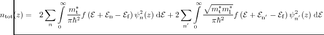
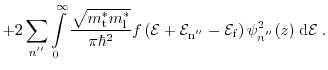
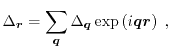
occupations, which leads to a modified carrier concentration. This concentration can be
obtained as
The subband occupation number is represented by the Fermi-Dirac distribution
function
 . After convergence is reached, which is achieved by an exchange of energy eigenvalues, wavefunctions,
and subband occupations, the transport parameters can be extracted.
. After convergence is reached, which is achieved by an exchange of energy eigenvalues, wavefunctions,
and subband occupations, the transport parameters can be extracted.
In Fig. 3.2, a result of the self-consistent loop between the
Schrödinger-Poisson solver and the MC simulator is presented.
Several velocities for different inversion layer concentrations
 as a function
of the lateral field for a UTB SOI MOSFET device with a channel thickness of
as a function
of the lateral field for a UTB SOI MOSFET device with a channel thickness of
 and a substrate doping
of
and a substrate doping
of
 have been extracted.
Figure 3.2:
Carrier velocity as a function of the driving field for different inversion
layer concentrations. Due to surface roughness scattering, the carrier
velocity decreases for increasing inversion layer concentrations. The maximum
velocity is below the saturation velocity of bulk Si.
|
|
Surface roughness scattering (SRS) is the main scattering process in high
inversion layer concentrations, which has a strong impact on the transport parameters (see Fig. 3.3).
Figure 3.3:
The effective mobility as a function of the effective
field [7]. For increasing bulk doping and for low inversion
layer concentrations Coulomb scattering is the main scattering process, while for
increasing
phonon scattering becomes more important.
|
|
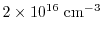
Surface roughness can be seen as a barrier at the interface,
whose position has a small and slowly varying displacement
 . Here,
 is the two-dimensional vector in the plane of the
interface [47].
is the two-dimensional vector in the plane of the
interface [47].
can be expressed by its Fourier components
 |
(3.2) |
whereas the power spectrum
 is usually
modeled with a Gaussian form as [155]
is usually
modeled with a Gaussian form as [155]
or with an exponential shape as described
in [156,157].
 is the difference between the incoming
wavevector
is the difference between the incoming
wavevector
 and the wavevector
 after the scattering event.
 is the correlation length of the oxide thickness fluctuations and should be
understood as the minimum distance between two points at which thicknesses are
considered independent.
The SRS matrix elements
is the correlation length of the oxide thickness fluctuations and should be
understood as the minimum distance between two points at which thicknesses are
considered independent.
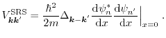
The SRS matrix elements
 have
been defined and discussed in [158] as
have
been defined and discussed in [158] as
Therefore, the derivative of the wave function at the interface plays an important
role. The quantization direction in equation (3.4) is in
 direction. In [47] it has been shown that the scattering potential
depends linearly on the inversion layer concentration
defined as [47,1]
direction. In [47] it has been shown that the scattering potential
depends linearly on the inversion layer concentration
defined as [47,1]
 |
(3.5) |
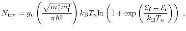
and on the depletion concentration
 which can be expressed as [7]
 |
(3.6) |
 and
and
 denote the substrate and the intrinsic concentration, respectively.
The influence of this dependence on higher-order transport parameters will be shown in the sequel.
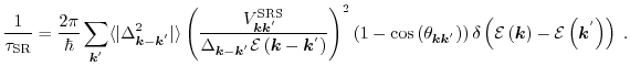
Inserting the scattering matrix into Fermi's golden rule (see
equation (1.137)) and integrating over the whole space, the SRS time
denote the substrate and the intrinsic concentration, respectively.
The influence of this dependence on higher-order transport parameters will be shown in the sequel.
Inserting the scattering matrix into Fermi's golden rule (see
equation (1.137)) and integrating over the whole space, the SRS time
 can be written as [47]
With a large correlation length
, the interface is locally flat and
therefore the term
 tends to zero, which
means that the surface roughness scattering is not effective. For
small
the relaxation time is determined by the product of
tends to zero, which
means that the surface roughness scattering is not effective. For
small
the relaxation time is determined by the product of  and
(see equation (3.3)). In fact, for relatively
small correlation lengths, a considerable scattering rate is observed, if the
amplitude of thickness variations
is high enough. The energy in the
denominator of the expression
and
(see equation (3.3)). In fact, for relatively
small correlation lengths, a considerable scattering rate is observed, if the
amplitude of thickness variations
is high enough. The energy in the
denominator of the expression
 reflects the
fact that scattering with small wave vectors predominates,
reflects the
fact that scattering with small wave vectors predominates,
 is the essential
component entering the relaxation time [1], while the delta
function is related to the elastic nature of the process.
is the essential
component entering the relaxation time [1], while the delta
function is related to the elastic nature of the process.
The main differences between bulk transport and transport in an inversion layer is
the occurrence of quantum mechanical effects such as quantum confinement,
subbands and SRS.
Due to quantum confinement, carriers cannot move in the direction
perpendicular to the interface. Thus, carriers have to be treated as a
two-dimensional gas, which has a considerable impact on the transport properties.
In Fig. 3.4, higher-order mobilities as a function of the
inversion layer concentration
are shown.
In a bulk MOSFET within low fields, the carrier mobility
 fits the measurement data of
Takagi [7,159] quite well, while a significant reduction
is observed in the quantized
channel region of a UTB SOI MOSFET [160].
fits the measurement data of
Takagi [7,159] quite well, while a significant reduction
is observed in the quantized
channel region of a UTB SOI MOSFET [160].
Figure 3.4:
Higher-order mobilities as a function of the inversion layer
concentration
for different lateral fields. For
high fields the difference of the mobilities decreases. For low fields
in a bulk MOSFET the carrier mobility is equal to the measurement
data of Takagi.
|
|
A considerable deviation of higher-order mobilities for low
and low fields can be observed, while for high fields this deviation
disappears. All mobilities are constant for high fields and are not affected anymore by SRS.
Figure 3.5:
Conduction band edge as a function of the position for different
inversion layer concentrations. For high
, the carriers are closer to
the interface and hence they are more affected by surface roughness
scattering than for low
.
|
|
Figure 3.6:
Conduction band and wavefunctions of a UTB SOI MOSFET for
different electric fields. Both the wavefunctions and subbands are shifted with increasing
lateral electric fields. The conduction band edge is affected by the change in
the subband occupations.
|
|
The reason for the constant mobilities for high fields can be explained
with Fig. 3.5 and Fig. 3.6.
In Fig. 3.5 the conduction band edge for several
is presented. Due to the band bending for increasing
, the carriers move closer to the interface, and therefore the influence
of SRS becomes stronger, which results in a lowering of the
mobilities. For high fields, the distance of the carriers to the interface
increases, which reduces the influence of SRS on the mobilities.
This is demonstrated in Fig. 3.6.
Here, the behavior of the conduction band edge together with the first two subbands
and their wavefunctions for different driving fields of
 and
and
 is presented. As pointed out before, there is a shift of the conduction band edge and subbands to lower
values for increasing driving fields. The result of this band edge shift is
that the wavefunction is shifted away from the interface, which means
that the probability of finding a carrier near the
interface decreases. As a consequence, the influence of surface characteristics on the
transport parameters decreases as well. Therefore, the effect of SRS on the mobilities
is drastically reduced for high fields.
is presented. As pointed out before, there is a shift of the conduction band edge and subbands to lower
values for increasing driving fields. The result of this band edge shift is
that the wavefunction is shifted away from the interface, which means
that the probability of finding a carrier near the
interface decreases. As a consequence, the influence of surface characteristics on the
transport parameters decreases as well. Therefore, the effect of SRS on the mobilities
is drastically reduced for high fields.
Figure 3.7:
Influence of surface roughness scattering on
,
 , and
, and
 as a function of the lateral field for different
. For low fields, surface roughness scattering has a
strong impact, while for high fields the mobilities are unaffected by SRS.
as a function of the lateral field for different
. For low fields, surface roughness scattering has a
strong impact, while for high fields the mobilities are unaffected by SRS.
|
|
Figure 3.8:
Ratio between the mobilities neglecting and considering SRS for high
and low
values as a function of the lateral field. For low
, the
mobilities are unaffected. The carrier mobility is more affected by SRS than the
higher-order mobilities.
|
|
This is visible in Fig. 3.7.
Here, higher-order mobilities as a function of the electric field for
different inversion layer concentrations have been calculated both with and without
surface roughness scattering. For fields above
 , the
effect of surface roughness scattering on the carrier mobility can be
neglected, while for the energy flux mobility and the second-order energy flux
mobility even at
the scattering process has only a minor
impact. Thus, higher-order mobilities are not so much affected by SRS as the carrier mobility.
, the
effect of surface roughness scattering on the carrier mobility can be
neglected, while for the energy flux mobility and the second-order energy flux
mobility even at
the scattering process has only a minor
impact. Thus, higher-order mobilities are not so much affected by SRS as the carrier mobility.
This is demonstrated in Fig. 3.8, where the ratios of higher-order mobilities with and
without SRS for high and low inversion layer concentrations
of
 and
and
 , respectively, are plotted.
The difference in the low
regime between the ratio curves of
and the higher-order mobilities is not as high as in the strong inversion regime. This can be explained as follow: Surface roughness scattering changes the
momentum relaxation time
, respectively, are plotted.
The difference in the low
regime between the ratio curves of
and the higher-order mobilities is not as high as in the strong inversion regime. This can be explained as follow: Surface roughness scattering changes the
momentum relaxation time
 and therefore the velocity, which is
proportional to
, is shifted to
lower values for increasing
(see Fig. 3.10).
Therefore, the antisymmetric part of the distribution function is reduced for high inversion
layer concentrations following that the distribution function becomes more
isotropic. The effect is that the impact of SRS on the energy flux is not as
high as on the carrier flux. This is pointed out in Fig. 3.9.
where the ratio of the momentum relaxation time and the energy-flux relaxation time
and therefore the velocity, which is
proportional to
, is shifted to
lower values for increasing
(see Fig. 3.10).
Therefore, the antisymmetric part of the distribution function is reduced for high inversion
layer concentrations following that the distribution function becomes more
isotropic. The effect is that the impact of SRS on the energy flux is not as
high as on the carrier flux. This is pointed out in Fig. 3.9.
where the ratio of the momentum relaxation time and the energy-flux relaxation time
 is presented. Due to the strong increase for high
of
compared to
, the higher-order mobilities, which are
proportional to the relaxation times, are not as effected by SRS as
.
is presented. Due to the strong increase for high
of
compared to
, the higher-order mobilities, which are
proportional to the relaxation times, are not as effected by SRS as
.
Figure 3.9:
Ratio of the momentum relaxation time
and energy
flux relaxation time
for different
as a function of the
driving field. Surface roughness scattering influences
more
than
, especially for high inversion layer concentrations.
|
|
Figure 3.10:
Influence of surface roughness scattering on the electron velocities for
different
. For decreasing
, SRS loses the influence on the
carrier velocity. Due to non-parabolic bands and quantization, the velocity
is below the saturation velocity of the bulk.
|
|
The dependence of
on
has an
impact on the carrier velocity as pointed out
in Fig. 3.10. There, the velocity for high inversion layer
concentration and low inversion layer concentration is shown. The difference in
the high field case between the carrier velocities
considering once SRS and neglecting SRS for the high inversion layer
concentration case is about
 , while the velocities in the
high and low
neglecting SRS respectively, yield the same result.
, while the velocities in the
high and low
neglecting SRS respectively, yield the same result.
Figure 3.11:
Influence of surface roughness scattering on
 and
and
 as a function of the kinetic energy of the carriers for
different
. Due to the elastic scattering nature of SRS, the
relaxation times are not affected by SRS.
as a function of the kinetic energy of the carriers for
different
. Due to the elastic scattering nature of SRS, the
relaxation times are not affected by SRS.
|
|
Figure 3.12:
Energy relaxation time (left side) and the second-order
relaxation time (right side) as a function of the inversion layer concentration for
different lateral electric fields. For a field
of
 and high
,
and
increase in
contrast to high-fields, where the energy relaxation time remain constant.
and high
,
and
increase in
contrast to high-fields, where the energy relaxation time remain constant.
|
|
Fig. 3.11 shows the energy
relaxation time and the second-order relaxation time as a function
of the kinetic energy of the carriers for low and high inversion layer
concentrations considering and neglecting SRS. Due to the elastic nature of SRS,
there is no change in the energy relaxation time and in the second-order relaxation time.
Figure 3.13:
First subband occupation of the unprimed, primed, and
double primed valleys as a function of the inversion layer concentration
for fields of
and
 .
Due to the light mass of the unprimed valley in transport direction, the subband occupation
number is higher than in the other valleys.
.
Due to the light mass of the unprimed valley in transport direction, the subband occupation
number is higher than in the other valleys.
|
|
In Fig. 3.12,
and
as a function of
for
different lateral electric fields are presented. As can be observed, the relaxation times
for high fields are constant except for a lateral field
of
 . There is a significant change in the second-order relaxation time. This can be explained
with Fig. 3.13, where the first subband occupation as a function
of
of the unprimed, primed, and double primed valleys for lateral
fields of
, and
. There is a significant change in the second-order relaxation time. This can be explained
with Fig. 3.13, where the first subband occupation as a function
of
of the unprimed, primed, and double primed valleys for lateral
fields of
, and
 is shown. Due to the
fast increase of the occupation number of the first subband
in the unprimed valley at
compared to the high-field
case, where the occupation is constant, the change in the second-order
relaxation times increases as well for high
.
is shown. Due to the
fast increase of the occupation number of the first subband
in the unprimed valley at
compared to the high-field
case, where the occupation is constant, the change in the second-order
relaxation times increases as well for high
.
Fig. 3.14 demonstrates the mobilities in
each valley and the total average mobility as a function of the channel
thickness. The mobilities are indirectly
proportional to the effective masses.
As has been pointed out in Fig. 1.10, the velocity of the unprimed
valley is high compared to the primed and double primed valleys. This is due to the light
conduction mass of the unprimed valley and therefore the mobility is also high
compared to the other valleys.
The maximum peak in the total average mobility is due to a high occupation of
the unprimed ladder for a thickness of
 as demonstrated in Fig. 3.15.
By increasing the channel thickness to
as demonstrated in Fig. 3.15.
By increasing the channel thickness to
 , the occupation of the
unprimed valley decreases and the occupation of the primed valley with the
heavy conduction mass increases. The total mobility curve has a minimum
at about
bulk thickness. At this value, the
occupation of the primed valley has its maximum. After the occupation of the
double primed valley starts to increase, the total mobility increases too, until
the occupation numbers of each valley reach a saturation value.
Furthermore, it has been reported in [155] that for ultra thin body devices the
carrier mobility is proportional to the device thickness to the power of six,
which is in good agreement with the results.
, the occupation of the
unprimed valley decreases and the occupation of the primed valley with the
heavy conduction mass increases. The total mobility curve has a minimum
at about
bulk thickness. At this value, the
occupation of the primed valley has its maximum. After the occupation of the
double primed valley starts to increase, the total mobility increases too, until
the occupation numbers of each valley reach a saturation value.
Furthermore, it has been reported in [155] that for ultra thin body devices the
carrier mobility is proportional to the device thickness to the power of six,
which is in good agreement with the results.
Figure 3.14:
Mobilities of the unprimed, primed, and double primed valleys, and
total average mobility as a function of the channel thickness.
At about
 , there is a maximum in the total mobility. This is
the point where the mobility of the unprimed valley is already high while the
carrier mobility of the remaining valleys is low.
, there is a maximum in the total mobility. This is
the point where the mobility of the unprimed valley is already high while the
carrier mobility of the remaining valleys is low.
|
|
Figure 3.15:
Populations of the unprimed, primed, and double primed valleys as
functions of the channel thickness.
|
|
3.4 Comparison with Bulk Simulations
To point out just the influence of quantization on higher-order transport
parameters, the subband results have been compared to three-dimensional bulk
data. Surface roughness scattering has not been considered in these subband simulations.
In Fig. 3.16,
,
, and
are compared to
bulk simulations with a doping of
 .
As can be observed, the higher-order mobilities of the 2D electron
gas are below the mobilities of the 3D bulk simulations, especially in the low field
regime.
.
As can be observed, the higher-order mobilities of the 2D electron
gas are below the mobilities of the 3D bulk simulations, especially in the low field
regime.
Figure 3.16:
Carrier, energy-flux, and second-order energy flux mobility of SMC and bulk MC simulations. The
mobilities obtained by bulk simulations are higher than in subband
simulations. For high fields, the mobilities from subband simulations
yield the same value as from bulk simulations.
|
|
Figure 3.17:
Comparison of the energy relaxation time and second-order energy
relaxation time using 2D SMC data and 3D bulk MC data. For high energies both
simulations converge to the same value.
|
|
This behavior can be explained as follows: Due to Heisenberg's
uncertainty principle, there is a wider distribution of momentum in the
quantization area, because of a higher localization of the particles than in
the bulk. Hence, there are more bulk phonons available that can assist the transition between electronic states.
This will lead to an increase of the phonon rates and a decrease of the mobilities [161].
Due to the higher probability of scattering with phonons in the subband case,
the energy relaxation time and the second-order energy relaxation time are
lower than in the bulk as demonstrated in Fig. 3.17. This is also
the case in the carrier temperatures as visualizes
in Fig. 3.18.
Here, the subband carrier temperature is below
the bulk temperature due to the fact, that an increase of the phonon scattering
probability decreases the carrier temperature. However, for high energies, the relaxation times and the
temperatures of the subband simulations converge to the
bulk results due to the occupation of higher subbands.
Figure 3.18:
Comparison of the carrier temperature using 2D SMC data and 3D bulk MC
data. Due to higher phonon scattering in the 2D case the temperature is lower
than in the 3D case.
|
|
Figure 3.19:
Subband occupations as functions of the subband ladders in the
unprimed, primed, and double primed valleys for electric fields
of
 and
. For
high fields, the subband ladders in the primed and double primed valleys are occupied.
and
. For
high fields, the subband ladders in the primed and double primed valleys are occupied.
|
|
Fig. 3.19 shows the subband occupation as a function of the subband
ladders for a low field and a high field. As pointed
out, for an electric field of
 , the first
subband in the unprimed valley is highly occupied, while the ladders in the
primed and double primed valleys are more or less unoccupied. The situation changes for
a field of
, the first
subband in the unprimed valley is highly occupied, while the ladders in the
primed and double primed valleys are more or less unoccupied. The situation changes for
a field of
 . The carriers gain more energy, which results in the occupation of
higher subbands. The occupation values of the first two ladders in the primed and double primed
valleys are higher than in the unprimed valley.
. The carriers gain more energy, which results in the occupation of
higher subbands. The occupation values of the first two ladders in the primed and double primed
valleys are higher than in the unprimed valley.
A study of the influence of important inversion layer effects on higher-order transport
parameters using the SMC method has been given. The investigations
made in this chapter are based on a homogeneous bulk subband system, where all
spatial gradients of the macroscopic transport models are negliable. The next chapter is
devoted to higher-order transport models in real devices.
Next: 4. Subband Macroscopic Models
Up: Dissertation Martin-Thomas Vasicek
Previous: 2. The Three-Dimensional Electron
M. Vasicek: Advanced Macroscopic Transport Models
![\includegraphics[width=0.5\textwidth]{figures/svg/Subb_MonteCarlo.eps}](img580.png)
![\includegraphics[width=0.5\textwidth]{rot_figures_left/simulation/transport/vmc2deg/velocity_utbsoi.eps}](img585.png)
![\includegraphics[width=0.5\textwidth]{figures/svg/scattering.eps}](img586.png)
![\includegraphics[width=0.5\textwidth]{rot_figures_left/conferences/sispad2008/mobtak0123.eps}](img607.png)
![\includegraphics[width=0.5\textwidth]{rot_figures_left/simulation/transport/vmc2deg/ec_confined.eps}](img608.png)
![\includegraphics[width=0.5\textwidth]{rot_figures_left/conferences/sispad2007/en2_color.ps}](img609.png)
![\includegraphics[width=0.5\textwidth]{rot_figures_left/simulation/transport/vmc2deg/mobility_surface.eps}](img611.png)
![\includegraphics[width=0.5\textwidth]{rot_figures_left/simulation/transport/vmc2deg/energy_mobility.eps}](img612.png)
![\includegraphics[width=0.5\textwidth]{rot_figures_left/simulation/transport/vmc2deg/sec_energy_mobility.eps}](img613.png)
![\includegraphics[width=0.5\textwidth]{rot_figures_left/simulation/transport/vmc2deg/ratiomob.eps}](img614.png)
![\includegraphics[width=0.5\textwidth]{rot_figures_left/simulation/transport/vmc2deg/tau_surf_nosurf.eps}](img618.png)
![\includegraphics[width=0.5\textwidth]{rot_figures_left/simulation/transport/vmc2deg/velocity_surface.eps}](img619.png)
![\includegraphics[width=0.5\textwidth]{rot_figures_left/simulation/transport/vmc2deg/tau1_surf_new.eps}](img620.png)
![\includegraphics[width=0.5\textwidth]{rot_figures_left/simulation/transport/vmc2deg/tau2_surf_new.eps}](img621.png)
![\includegraphics[width=0.5\textwidth]{rot_figures_left/conferences/sispad2008/relax_Elat.ps}](img622.png)
![\includegraphics[width=0.5\textwidth]{rot_figures_left/conferences/sispad2008/relax2_Elat.ps}](img623.png)
![\includegraphics[width=0.5\textwidth]{rot_figures_left/conferences/sispad2008/subbandocc_2.eps}](img624.png)
![\includegraphics[width=0.5\textwidth]{rot_figures_left/conferences/sispad2007/channelthickness.eps}](img627.png)
![\includegraphics[width=0.5\textwidth]{rot_figures_left/simulation/transport/vmc2deg/subb_occupation_thickness.eps}](img628.png)
![\includegraphics[width=0.5\textwidth]{rot_figures_left/conferences/sispad2007/mue0_bulk_subb.eps}](img629.png)
![\includegraphics[width=0.5\textwidth]{rot_figures_left/conferences/sispad2007/mob1_subb_mob.eps}](img630.png)
![\includegraphics[width=0.5\textwidth]{rot_figures_left/conferences/sispad2007/mob2_subb_mob.eps}](img631.png)
![\includegraphics[width=0.5\textwidth]{rot_figures_left/conferences/sispad2007/tau1_bulk_subb.eps}](img632.png)
![\includegraphics[width=0.5\textwidth]{rot_figures_left/conferences/sispad2007/tau2_bulk_subb.eps}](img633.png)
![\includegraphics[width=0.5\textwidth]{rot_figures_left/conferences/sispad2007/temp_bulk_subb.eps}](img634.png)
![\includegraphics[width=0.5\textwidth]{rot_figures_left/simulation/transport/vmc2deg/pop_ev_1.eps}](img635.png)
![\includegraphics[width=0.5\textwidth]{rot_figures_left/simulation/transport/vmc2deg/pop_ev_100.eps}](img636.png)