


Next: 4.2.3 Random Number Generator
Up: 4.2 Code structure
Previous: 4.2.1 Graphical User Interface
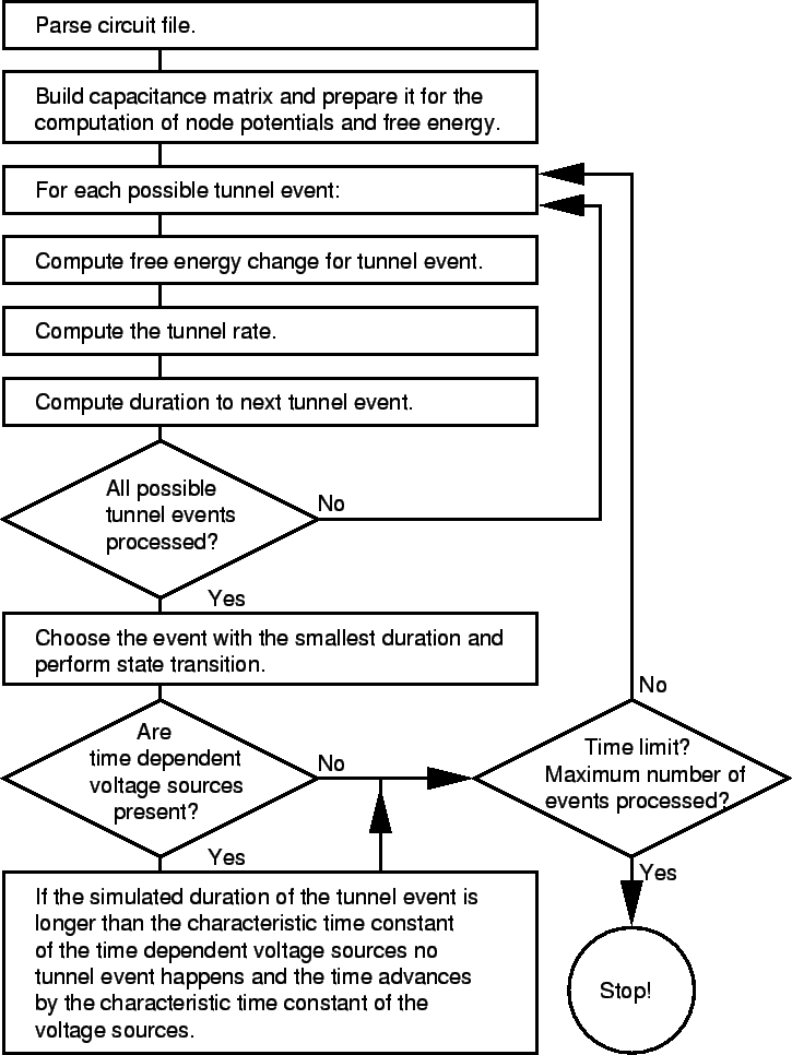
The important steps SIMON is going through during a simulation run are shown
in the flow chart in Fig. 4.4.
A parser written in
lex/yacc [77] reads in the circuit description and stores the
information in linked lists. Then the equation system linking known
Figure 4.4:
Flow chart of the inner loop of SIMON.
|
quantities with unknown ones are assembled. Afterwards the inner loop is
entered
where change in free energy, tunnel rate and the exponentially
distributed duration between tunnel events for each possible event are
computed. The event with the smallest duration is the winner and is
used to compute the new state of the circuit. In the case of a
transient
simulation with time dependent
voltage sources one more test has to be passed before the time is advanced and
a new event is simulated. If the
duration to the next tunnel event is
bigger
than a user defined time constant
 ,
which should be smaller
than the smallest characteristic time constant of the voltage sources, no
tunnel event takes place and the time is only advanced by the user defined time
constant
.
A good choice for
is
,
which should be smaller
than the smallest characteristic time constant of the voltage sources, no
tunnel event takes place and the time is only advanced by the user defined time
constant
.
A good choice for
is
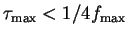 ,
where
,
where
 is the
maximum frequency of any voltage source present. A too
long duration to the next tunnel event means
that in the computed tunnel interval the voltage sources have changed
considerably which demands a recalculation of tunnel rates.
In Fig. 4.5 one can see that if the smallest time
between two tunnel events,
is the
maximum frequency of any voltage source present. A too
long duration to the next tunnel event means
that in the computed tunnel interval the voltage sources have changed
considerably which demands a recalculation of tunnel rates.
In Fig. 4.5 one can see that if the smallest time
between two tunnel events,  ,
is too big, the interval has to be
partitioned into smaller steps
,
is too big, the interval has to be
partitioned into smaller steps  .
.
Figure 4.5:
If the characteristic time constant of time dependent voltage sources
is smaller than the duration to the next tunnel event, a finer time
resolution has to be chosen to achieve more accurate transient behavior.
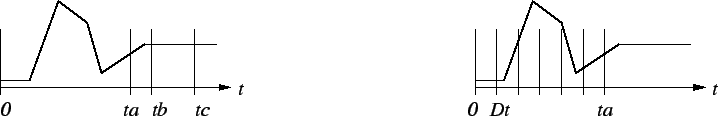 |
Therefore the time is advanced only
by ,
time dependent voltage sources are updated, and a new event is
computed. In this way transient behavior is simulated more
accurately. This method preserves the statistics of tunneling accurately to
the first order. The probability that a tunnel event happens sometime
before
is
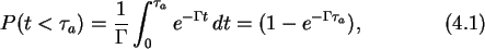
where the factor  in front of the integral is a normalization factor
to make the probability unity for
in front of the integral is a normalization factor
to make the probability unity for
 .
The probability
that the event happens in the short time
is thus
.
The probability
that the event happens in the short time
is thus
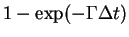 .
If
is split up into n intervals
long, one gets for the probability
that the event happens within
.
If
is split up into n intervals
long, one gets for the probability
that the event happens within 
which is correct to the first order with (4.1).
Next: 4.2.3 Random Number Generator
Up: 4.2 Code structure
Previous: 4.2.1 Graphical User Interface
Christoph Wasshuber