∕dy, with the work, d
 ∕dy, done
by the misfit stress, σijm, in forming the unit length of a dislocation along the
film–substrate interface. As a consequence, the critical thickness criterion is given
by
∕dy, done
by the misfit stress, σijm, in forming the unit length of a dislocation along the
film–substrate interface. As a consequence, the critical thickness criterion is given
by
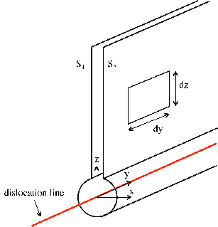
The system shown in Figure 4.1 is composed of a thin film with a finite thickness in the
region 0 < z < h, and a semi-infinite substrate filling the half space z < 0. The dislocation is
along the interface z = 0 aligned along the y-axis. The critical thickness criterion
compares the dislocation energy per unit length, d∕dy, with the work, d∕dy, done
by the misfit stress, σijm, in forming the unit length of a dislocation along the
film–substrate interface. As a consequence, the critical thickness criterion is given
by
 | (4.1) |
| Figure 4.1: | The straight infinitely long dislocation at the film–substrate interface. The film thickness is h, the slip plane is tilted by an angle ϕ from the normal to the interface. |
Since the film is much thinner than the semi-infinite substrate, the strain in the substrate is assumed to be zero while the complete lattice mismatch is accommodated in the film (i.e., any mismatch strain relaxation by substrate bending is neglected). According to the geometry shown in Figure 4.1, the top surface z = h of the film is traction free and therefore σxzm(x,h) = σ zzm(x,h) = σ yzm(x,h) = 0. Assuming all directions within the xy-plane (the hexagonal plane) are equivalent, a planar stress state is obtained and thus the mismatch strain components are εxxm = ε yym = ε m, where εm is the misfit strain, defined as
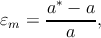 | (4.2) |
considering that the thin film’s in-plane lattice constant a adjusts to the rigid substrate’s lattice constant a*.
Hooke’s law (2.10) for isotropic structures reads
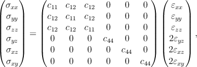 | (4.3) |
where c44 =  ∕2. In the case of cubic and hexagonal symmetries, the shape of the
stiffness matrix cij changes to
∕2. In the case of cubic and hexagonal symmetries, the shape of the
stiffness matrix cij changes to
 | (4.4) |
respectively, where c66 = (c11 - c12)∕2 for the hexagonal symmetry (the right matrix above).
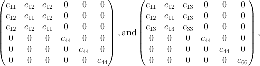
Considering for example the hexagonal symmetry, Hooke’s law gives
 | (4.5) |
which results in
 | (4.6) |
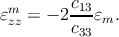
Finally, Hooke’s law yields for the mismatch stress
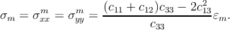 | (4.7) |
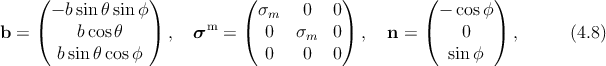
In the chosen Cartesian coordinate system, the Burgers vector b, the tensor of the misfit stress σm, and the outer normal to the cut surface Γ = S 2 + S4 (see Figure 3.1) denoted by n take the forms
 ∕dy, done by the misfit stress is calculated
according to [19]
∕dy, done by the misfit stress is calculated
according to [19]
 = = | ∫
0h∕cosϕ ∑
i,jbiσijmn
jdz = ∫
0h∕cosϕ ∑
i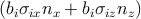 dz dz | ||
| = | bσmh sin θ sin ϕ. | (4.9) |
The formula for the dislocation energy dd∕dy for a straight dislocation inside an infinite
isotropic medium reads [19,23,32]:
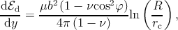 | (4.10) |
where μ and ν are the shear modulus and the Poisson ratio, respectively, φ is the angle between the Burgers vector b and the dislocation line, and R is the outer cut-off radius. Here it is taken to be equal to the film thickness.
Chapter 3.2 describes how to calculate the dislocation energy dd∕dy inside an infinite
anisotropic medium according to the procedure developed by Steeds [72] and described in
Section 3.4:
 | (4.11) |
where K is the pre-logarithmic factor and it is a function of the crystal structure and the elastic properties (see Section 3.4). Holec [25] derived a simplified expression of K from the Steeds procedure specifically for a dislocation along the y-axis inside a hexagonal crystal. The expression is easily adapted to the cubic symmetry by simply modifying the stiffness tensor.
If we want to calculate the dislocation energy at the interface between the film and the substrate of a heteroepitaxial structure, it is necessary to evaluate the effect of the free surface of the film and the different elastic properties of the two materials. Willis, Jain and Bullough [82] have evaluated both effects on the dislocation energy within isotropic elasticity.
The adaptation of the Willis, Jain and Bullough model to the hexagonal symmetry can be found in the works of Holec [24] and Coppeta [8]. This procedure is reported in details in the next Paragraph 4.2.3 for a straight dislocation at the interface between a finite hexagonal film and a semi-infinite hexagonal substrate with different elastic constants.
In conclusion, four approaches (summarized in Table 4.1) for calculating the dislocation energy were defined above, which will be used to evaluate the impact of different approximations.
The evaluation of the integrals along the surfaces S2 and S4 (see Figure 3.1) deals with a straight dislocation at the interface between a finite anisotropic film and a semi-infinite anisotropic substrate with different elastic properties:
 | (4.12) |
Considering Figure 4.2, the previous equation becomes
 | (4.13) |
If the extremes of the second integral are inverted, one obtains
 | (4.14) |
where ui(x → 0+) - u
i(x → 0-) = b
i.
The evaluation of the stress components in (4.14) is performed through the treatment
suggested by the Willis, Jain and Bullough model [82] for hexagonal and cubic symmetries
following the Steeds procedure [72].
| Figure 4.2: | The z-axis is perpendicular to the c-plane for the hexagonal symmetry and to the closed packed plane for the cubic one. The dislocation line lies along the y-axis in both cases. |
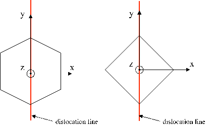
| Figure 4.3: | The z-axis is perpendicular to the c-plane for the hexagonal symmetry and to the closed packed plane for the cubic one. The dislocation line lies along the y-axis in both cases. |
The dislocation of interest is a misfit dislocation along the c-plane of the wurtzite structure or the closed packed plane of the diamond structure. The z-axis is perpendicular to the c-plane or to the closed packed plane, respectively (See Figure 4.3). The dislocation is considered straight and extended to infinity along the y-axis. This assumption simplifies the problem to a plane strain problem where no quantity depends on the y-coordinate, so
 | (4.15) |
The Burgers vector of the dislocation is b. Displacements are given by the functions ux, uy and uz. The displacements ux and uz correspond to the edge component of the considered dislocation whereas uy corresponds to the screw component. The strain components are
εxx =  ,εxy = ,εxy =   , , | |||
εyy = 0,εxz =  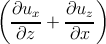 , , | (4.16) | ||
εzz =  ,εyz = ,εyz =   . . |
The fact that εyy = 0 yields a relation between particular stress components:
 | (4.18) |
The compliances reflecting the proper hexagonal symmetry have been used to obtain:
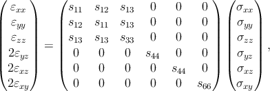 | (4.19) |
where
 | (4.20) |
The shape of the tensor for cubic symmetry (in both Si(100) and Si(110)) is the same as for the hexagonal one. The subsequent treatment is valid for the cubic symmetry with s66 = s44 and s13 = s12.
According to the Willis, Jain and Bullough model, it is useful now to have the jumps in
displacements occur over a surface which is perpendicular to the free surface instead of
across the slip plane. All quantities in the substrate have a * superscript to distinguish them
from quantities related to the thin film. The Fourier transform of a function f is denoted by
 . It is possible to split the problem into two independent parts, resolving the edge and the
screw components separately.
. It is possible to split the problem into two independent parts, resolving the edge and the
screw components separately.
The displacement field in the thin film can be decomposed into
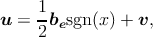 | (4.21) |
where be =  and the function v is continuous for all x. The strain field (and
thus also the stress field) inside the thin layer is determined only by the v part
as (except at the cut surface x = 0) the derivatives of the sgn(x) function are
equal to zero everywhere. To solve this problem, Fourier-transformed variables are
employed:
and the function v is continuous for all x. The strain field (and
thus also the stress field) inside the thin layer is determined only by the v part
as (except at the cut surface x = 0) the derivatives of the sgn(x) function are
equal to zero everywhere. To solve this problem, Fourier-transformed variables are
employed:
 | (4.22) |
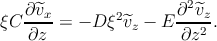
The Fourier transform of the ∂∕∂x operator is -iξ. Using (4.21) and (4.16), the Fourier components of the strain tensor are:
The equilibrium conditions [72] take the form
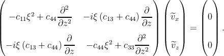
Transforming these equations into their Fourier equivalents and using Hooke’s law with
the stiffness tensor gives the following system of partial differential equations for the
Fourier-transformed components of the displacements  x and
x and  z:
z:
 | (4.25) |
In order to simplify the notation, the quantities A = -c11 , B = c44, C = -i(c13 + c44), D = -c44, E = c33 are introduced. From the second equation of the system one obtains
 | (4.26) |
Using this equation and its twice differentiated form with respect to z and substituting them into the first equation of the system (4.25), which is once differentiated with respect to z, yields
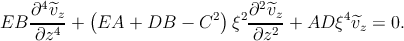 | (4.27) |
The solution has the exponential form eλ z. The corresponding proper λs are solutions of
the characteristic equation
z. The corresponding proper λs are solutions of
the characteristic equation
 | (4.28) |
The solutions are λ1 = κ1, λ2 = -κ1, λ3 = κ2 and λ4 = κ2, where
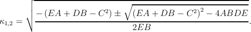 | (4.29) |
Therefore, the general solution to (4.27) has the form [72]
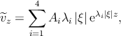 | (4.30) |
where Ai are functions of ξ to be determined. The component  x can then be obtained
from (4.26). Its general solution is
x can then be obtained
from (4.26). Its general solution is
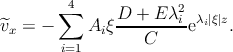 | (4.31) |
Evidently
 | (4.32) |
The Fourier-transformed components of the strain tensor are now easy to obtain from combining Equations (4.30), (4.31), and (4.23):
Using Hooke’s law, which has the same form when Fourier transformed, one obtains:
 xx xx | = c11 xx + c13 xx + c13 zz = -∑
i=14A
iξ2λ
i2c
44 zz = -∑
i=14A
iξ2λ
i2c
44 eλi eλi z, z, | (4.34a) |
 xz xz | = 2c44 xz = -∑
i=14iA
i xz = -∑
i=14iA
i ξλic44 ξλic44 eλi eλi z, z, | (4.34b) |
 zz zz | = c13 xx + c33 xx + c33 zz = ∑
i=14A
iξ2c
44 zz = ∑
i=14A
iξ2c
44 eλi eλi z, z, | (4.34c) |
where the identity c11c44 +  λi2 + c
44c33λi4 = 0 was used in the
expression for
λi2 + c
44c33λi4 = 0 was used in the
expression for  xx.
xx.
The general solution for the substrate region takes the same form (except that all variables have a star superscript). It is assumed that the substrate is not influenced by the thin layer as z →-∞. To fulfill this condition, the constants A2* and A 4* must be identically zero. Boundary conditions must be employed now in order to determine the constants A1, A2, A3, A4, A1*, and A 3*.
The Fourier transform of 1∕2sgn(x) is i∕ . The continuity of displacements across
the interface z = 0 is expressed by the following equations:
. The continuity of displacements across
the interface z = 0 is expressed by the following equations:
which result in the equations
where the notation
Γi =  ,Γi* = ,Γi* =  ,i = 1, 2. ,i = 1, 2. | (4.37) |
The second set of equations is obtained from the requirement that tractions must be continuous across the interface z = 0:
Combining Equations (4.34) and (4.38) gives
where the simplifying notation
Λi = 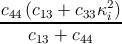 ,Λi* = ,Λi* =  ,i = 1, 2, ,i = 1, 2, | (4.40) |
The condition  xz
xz = 0 is expressed as
 κ
1Λ1 + κ
1Λ1 +  κ
2Λ2 = 0 κ
2Λ2 = 0 | (4.41) |
 zz
zz = 0 yields
 Λ
1 + Λ
1 +  Λ
2 = 0. Λ
2 = 0. | (4.42) |
 xx,
xx,  xz and
  zz, respectively, with the substituted
resolved constants A1,...,A4.
zz, respectively, with the substituted
resolved constants A1,...,A4. The procedure for the screw component is similar but simpler. The Burgers vector of a
screw dislocation has only one non-zero component, by, and thus the only non-zero
component of the displacement is uy. Moreover, it is again a plane strain problem, i.e.,
∂∕∂y = 0. As a consequence, the only non-zero strain components are εxy and εyz.
Similarly to the case of the edge dislocation, it is more convenient to deal with the
Fourier-transformed component  y rather than with uy itself. The Fourier-transformed
components of the strain are
y rather than with uy itself. The Fourier-transformed
components of the strain are
and the FT stress components obtained from Hooke’s law are
The equilibrium condition [72]
 + +  = 0 = 0 | (4.45) |
 y:
y:
- ξ2c
66 y y + c44 + c44  = 0, = 0, | (4.46) |
 y = A1e y = A1e
 z
+ A2e- z
+ A2e-  z
. z
. | (4.47) |
Values of A1 and A2 fulfilling these equations are
The stress components can be obtained by the inverse Fourier transform of  xy and
  xz
with the substituted A1 and A2 from the last two equations.
xz
with the substituted A1 and A2 from the last two equations.
After that, the components of the stress and the Burgers vector can be substituted in (4.14) to calculate the dislocation energy.
According to equation (4.1), equating the work done by the misfit strain with each of the four formulas for dislocation energy yields four different models with which to calculate the equilibrium critical thickness . These models are summarized with the respective hypotheses in Table 4.1 and their results are discussed in the subsequent Paragraphs. In particular, the critical thickness model developed by Freund [17], which neglects the differences between film and substrate, considers only isotropic elasticity, and in its simplified (often used) formula also neglects the effect of the free surface. The Freund model is corrected for the elastic anisotropy using the Steeds treatment for the dislocation energy [72]. The fully isotropic model, but with the free surface and different elastic constants in the film and the substrate, employs the Willis, Jain and Bullough formula [82]. Finally, a model addressing all effects [8,24] is reported in Paragraph 4.2.3.
| Table 4.1: | An overview of different assumptions for evaluating misfit dislocation energy, and equilibrium critical thickness . |
| Freund | Steeds | Willis et al. | Steeds + Willis et al. | |
| [17,19] | [72] | [82] | [8,24] | |
| Anisotropy | no | yes | no | yes |
|
| no | no | yes | yes |
| Free surface of the film | no | no | yes | yes |
 +
+  = 2
= 2

 = 0
= 0


 (
(

 +
+  = 0
= 0 +
+  = 0
= 0
 e
e


 e
e


 +
+  =
= 


 +
+  =
= 

 Γ
Γ Γ
Γ =
= 

 =
= 
 =
= 


 =
= 


 Λ
Λ Λ
Λ


 =
= 
 =
=