2.3 Surface Kinetics

Once the particle transport to the surface is computed, the etch or deposition rate can be determined, which gives the desired surface velocity. In this work the arrival flux distributions are assumed to be in a pseudo-steady state. They only depend on the surface profile and the arrival flux distribution at plane ${\mathcal {P}}$ and not on their history. The surface velocity ${V}({\vec{x}})$ with ${\vec{x}}\in{\mathcal{S}}$ can be written as a functional of the local arriving flux distribution ${\Gamma}({\vec{x}})$

$${V}({\vec{x}}) = {V}({\Gamma}({\vec{x}})) .$$ (2.23)

For the numerical representation of the continuous flux distribution ${\Gamma}$ some form of discretization is required. If the functions ${r}_l({\vec{x}};{q},{\vec{\omega}},{E})$ with $1\leq l\leq {{N}_\text{R}}$ are appropriate weight functions which map ${\Gamma}({\vec{x}})$ to a finite number of scalar values given by

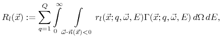$${R}_l({\vec{x}}):= \sum_{{q}=1}^{{Q}} \int\limits_{0}^{\infty} \i... ...\omega}},{E}) {\Gamma}({\vec{x}};{q},{\vec{\omega}},{E}) \,{d}{\Omega}\,{d}{E},$$ (2.24)

the surface velocity can be written as a function of these scalars

$${V}({\vec{x}}) = {V}({R}_1({\vec{x}}),{R}_2({\vec{x}}),\ldots,{R}_{{N}_\text{R}}({\vec{x}})) .$$ (2.25)

To save memory it is necessary to minimize the number of discretized values ${{N}_\text{R}}$ that need to be stored for each surface point. In Section 5.2 a method will be presented which does not require a discretization of the flux distribution in order to calculate the particle transport. Hence, the choice of weight functions must be appropriate primarily for an accurate calculation of the surface velocity.

Luckily, most models require only a minimum number of weight functions ${r}_l$ . Typically, all the information needed from the flux distribution ${\Gamma}$ for a certain particle type can be mapped to a single value representing a certain rate using a single weight function. This is not surprising, since only the total flux, in case of neutrals, or the effective sputter yield, in case of high energy ions, is required for common process models. The total flux ${F}_{{q}'}({\vec{x}})$ of particles of species ${q}'$ is obtained by choosing ${r}_l({\vec{x}};{q},{\vec{\omega}},{E}):=\delta_{{q}{q}'}$ which yields

$${R}_l({\vec{x}}) = \int\limits_{0}^{\infty} \int\limits_{{\vec{\o... ...vec{x}};{q}',{\vec{\omega}}, {E}) \,{d}{\Omega}\,{d}{E} = {F}_{{q}'}({\vec{x}})$$ (2.26)

For particles with higher kinetic energies, which are generally ions, the total flux is of less interest. The contribution of such particles to the surface velocity depends on the incident angle ${\theta}$ and energy ${E}$ and is described by a yield function ${Y}({\theta},{E})$ as introduced in Section 2.2.3. The total sputter rate ${Y}^{{\text{tot}}}_{{q}'}({\vec{x}})$ for particles of species ${q}'$ can be obtained by choosing ${r}_l({\vec{x}};{q},{\vec{\omega}},{E}):=\delta_{{q}{q}'}{Y}({\theta},{E})$

$${R}_l({\vec{x}}) = \int\limits_{0}^{\infty} \int\limits_{{\vec{\o... ...Y}({\theta},{E}) \,{d}{\Omega}\,{d}{E} = {Y}^{{\text{tot}}}_{{q}'}({\vec{x}}) .$$ (2.27)

Generally, all the ${R}_l$ values represent a rate on the surface, such as flux or total sputter rate of a certain particle species. Therefore, from now on, they will be interpreted as surface rates. The surface velocity ${V}$ is a function of these surface rates.