To demonstrate the ray tracing technique for surface rate calculation, a deposition process was applied to the initial structure given in Figure 4.5a. The structure was resolved on a grid with lateral grid extensions
![]() . A total of 25 million particles were simulated at every time step. The arrival flux distribution at the source plane was assumed to follow (2.5) with
. A total of 25 million particles were simulated at every time step. The arrival flux distribution at the source plane was assumed to follow (2.5) with
![]() . The sticking probability was 0.5 and diffusive reemission was assumed (2.18). For each incident particle, a new one was reemitted as long as the weight factor of the new particle was larger than 0.01 (
. The sticking probability was 0.5 and diffusive reemission was assumed (2.18). For each incident particle, a new one was reemitted as long as the weight factor of the new particle was larger than 0.01 (
![]() , see Section 5.2).
, see Section 5.2).
For the CFL criterion required by the LS method,
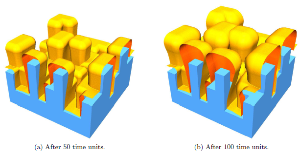
![]() was chosen. The results after a process time of 50 and 100 time units are shown in Figure 5.5. The simulation was carried out on 16 cores of AMD Opteron 8435 processors (
was chosen. The results after a process time of 50 and 100 time units are shown in Figure 5.5. The simulation was carried out on 16 cores of AMD Opteron 8435 processors (
![]() ). Different ray tracing data structures and splitting strategies were tested. Table 5.1 summarizes the average times which are spent on setting up the data structure and on ray tracing at each time step. The average memory consumption is also listed.
). Different ray tracing data structures and splitting strategies were tested. Table 5.1 summarizes the average times which are spent on setting up the data structure and on ray tracing at each time step. The average memory consumption is also listed.
Best runtimes have been observed for the SAH with
![]() . It should be noted that the measured times also include the costs for disk and surface intersection tests and for the random direction generation, which are identical for all data structures. Hence, the computational savings due to the ray tracing data structures are manifested by the measured values.
. It should be noted that the measured times also include the costs for disk and surface intersection tests and for the random direction generation, which are identical for all data structures. Hence, the computational savings due to the ray tracing data structures are manifested by the measured values.
The results clearly show that the ray tracing data structures are superior to the full grid which exhibits a much longer calculation time. The full grid stores a single link for every cell. In the case of a non-empty cell, this link gives access to its data. The bad scaling behavior, which is linear with the domain size, leads to a high memory consumption for larger structures.
The memory requirements for trees are much lower, because they are expected to scale linearly with the surface size. The applied ray tracing algorithm requires for each leaf the minimum and maximum indices of its bounding box. Furthermore, links to the two child nodes as well as the position and orientation of the splitting plane are needed. Finally, parent links must be stored for all nodes to enable up traversals within the tree.
The neighbor links arrays cannot compete with the kd-tree concerning memory consumption. However, the former shows better runtimes for most tested geometries. A likely reason for the good runtime performance is that the data structure clearly separates the neighbor links for positive and negative grid directions. Hence, depending on the direction of the ray, only the corresponding positive or negative array must be accessed. Since runtime, and not memory consumption, is the major concern for most topography simulations using ray tracing, the neighbor links arrays using SAH with
![]() are used for all simulations presented in Chapter 6.
are used for all simulations presented in Chapter 6.
The parallel efficiency of the surface rate calculation procedure was also tested on machines with four AMD Opteron 8435 six-core processors and AMD Opteron 8222 SE dual-core processors clocking at
![]() and
and
![]() , respectively. The average calculation time for rate calculation, using different numbers of cores, are listed in Table 5.2. The numbers refer to the neighbor links arrays data structure using SAH with
, respectively. The average calculation time for rate calculation, using different numbers of cores, are listed in Table 5.2. The numbers refer to the neighbor links arrays data structure using SAH with
![]() .
.
The parallel ray tracing algorithm is essentially just a loop whose independent iterations are distributed over all CPUs. Therefore, losses due to synchronization of threads can be neglected. Furthermore, memory access is read-only except for the surface rates. Each core has its own copy of the surface rates, which are finally summed up, in order to avoid concurrent write accesses. As a consequence, the memory bandwidth is the main crucial factor for the parallel efficiency, due to the random memory access pattern of the ray tracing algorithm. The efficiency is worse on the machine using six-core processors than on that using dual-core processors, because more cores must share the common connection to the main memory. This bottleneck is a well-known problem of today's multi-core processors [130].
![$\textstyle \parbox{\textwidth}{
\small
\begin{tabular}{
l
l
S[tabformat=2.2]
S[...
...nd} & 55.3\,\si{\second} & 197.0\,\si{\mega\byte}\\
\bottomrule
\end{tabular}}$](img695.png)
![$\textstyle \parbox{\textwidth}{
\small
\begin{tabular}{
S
S[tabformat=2.1]
S[ta...
...\si{\second} & 60.4\,\si{\percent} & {--} & {--} \\
\bottomrule
\end{tabular}}$](img697.png)