3 Approximative Shared-Memory Graph Coloring Algorithms
As graphs can model any kind of relationship between various entities they occur in many different fields of practical applications and research, such as computational science and engineering [34], [101], [102], social network analysis [28], data mining [103], linear algebra [104], [105], and mesh adaptation [18], [29], [30], [31]. One prominent graph problem is the decomposition of a computational problem into (independent) sub-problems which can be executed in parallel with a minimum of inter-sub-problem dependencies. This decomposition task can be described as a distance-1 graph coloring problem (see Section 2.1.1). In general, there exist two types of solutions to the aforementioned problem: An exact and optimal solution, which can be hard to derive, and an approximative nearly-optimal solution, which is computationally less expensive to obtain. For both types various different approaches and algorithms are available.
A major difference between exact and inexact algorithms, besides their solution quality, is represented by their runtime. An exact algorithm will most likely spend more time on exploring the solution space, as compared to an inexact algorithm. Therefore, inexact algorithms are used to approximately solve the graph coloring problem. Especially for large-scale problems, the main focus is on decomposing the computational problem at hand into smaller parts of work, which can subsequently be processed simultaneously (as much as possible). Thus, a fast graph coloring solution approach is necessary to avoid that the problem decomposition step becomes an unwanted bottleneck, jeopardizing the overall computational performance.
The aim of this chapter is the evaluation of available approximative serial and shared-memory parallel graph coloring algorithms for the distance-1 graph coloring problem. These algorithms form the basis of the developed parallelization approaches presented in the subsequent Chapters 4 and 5. One of the constraints in solving the graph coloring problem is to minimize the number of used colors \(k\) necessary for a feasible coloring. A major drawback of this constraint is often neglected: The highly different population of the resulting color classes. It can happen, for example, that the applied graph coloring algorithm terminates with the smaller color classes having the largest population counts compared to higher color classes [33]. Considering computational performance for a given task represented by the graph, such heavily unbalanced color classes lead to computational load-imbalance, reducing the parallel efficiency of the overall parallel implementation.
Multiple approaches have been presented on comparing different approximative graph coloring algorithms [28], [106], [107], [108]. However, the here presented overview includes recent developments presented in the field of graph coloring. Therefore, the results of a literature review on graph coloring algorithms, focusing on shared-memory approaches, are presented in Section 3.1. Section 3.2 is dedicated to give an overview on the investigated algorithms in this work [109], [110]. Additionally, the choice of the specific algorithms is argued. The used set of test graphs and the obtained benchmarking results are also discussed in Section 3.2. Finally, an overview on the results and a short outlook on future research is given in Section 3.3.
3.1 Related Work
3.1.1 Exact Algorithms
Although the problem of finding an optimal coloring of a given graph is NP-complete, several methods have been introduced which aim at finding this optimal solution faster than a blindingly straightforward search approach. One example of an exact algorithm is the tree-based backtracking approach, which is, in general, a method used to determine the optimal solution of any kind of problem [111]. Its main idea is to create partial solutions and subsequently combining them into a complete solution. A partial solution is refused if it is sure that it cannot be evolved into an optimal solution. Backtracking algorithms perform better for the graph coloring problem if an ordering of the graph vertices is considered beforehand, e.g., ordering in decreasing order of degree [33].
Another option of exactly solving the graph coloring problem is the use of a special type of linear programming model, i.e., integer programming (IP). A basic IP formulation of the graph coloring problem using a graph \(G(V,E)\) is based on two matrices \(\mathbf {X}_{n \times n}\) and \(\mathbf {Y}_n\) holding only integers. The entries of the two matrices denote the colorings of the vertices and if a specific color class is populated at all.
\( \seteqsection {3} \)
\begin{equation} X_{ij} = \begin {cases} 1, \ \text {if} \ c(v_i)=j \\ 0, \ \text {otherwise} \end {cases} \end{equation}
\( \seteqsection {3} \) \( \seteqnumber {2} \)
\begin{equation} Y_j = \begin {cases} 1, \ \text {if the number of vertices with} \ c(v)=j \geq 1 \\ 0, \ \text {otherwise} \end {cases} \end{equation}
With these two matrices the graph coloring problem can be formulated as an optimization problem, minimizing the necessary number of colors
\( \seteqsection {3} \) \( \seteqnumber {3} \)
\begin{equation} \text {min}\sum _{j=1}^{n}Y_j, \end{equation}
with respect to
\( \seteqsection {3} \) \( \seteqnumber {4} \)
\begin{equation} X_{ij}+X_{lj} \leq Y_j, \ \ \forall \ \{v_i,v_l\} \in E, \ \forall \ j \in \{1,...,n\}, \label {eq:graph_coloring:exact:constraint1} \end{equation}
\( \seteqsection {3} \) \( \seteqnumber {5} \)
\begin{equation} \sum _{j=1}^{n}X_{ij}=1, \ \ \forall \ v_i \in V. \label {eq:graph_coloring:exact:constraint2} \end{equation}
The first constraint (Equation 3.4) ensures that adjacent vertices do not belong to the same color class, whereas the second constraint defined by Equation 3.5 states that a vertex can only be present in one color class [33]. Graph coloring methods utilizing integer programming have been presented by, e.g., Zais and Laguna [42], Hertz et al. [112], Thevening et al. [113], and Jabrayilov and Mutzel [114].
3.1.2 Approximative Algorithms
As the runtimes of exact algorithms are considerably longer due to the complexity of the graph coloring problem than the subsequent computations conducted on the created independent sets represented by the graph vertices, it is often more practicable to apply approximative algorithms [33]. A straightforward solution approach of the graph coloring algorithm is represented by the Greedy coloring algorithm [115], [116]. This algorithm uses a strategy called first-fit, where the vertices of the graph are assigned the smallest color possible, by checking all colors assigned to the adjacent vertices. Hence, for any given graph \(G(V,E)\) the algorithm uses a maximum of \(\Delta (G)\) colors. Regarding the population of the color classes, the Greedy algorithm assigns the smaller colors way more often than the higher colors, yielding a highly skewed population distribution of the color classes. Nevertheless, the resulting coloring of any graph depends heavily on the ordering of the vertices, but it often delivers well enough or sometimes even optimal results [33].
Applying a different heuristic for choosing the actual color that is to be assigned to a vertex leads to a better distribution of the color class populations. One way to achieve this is to assign the permissible color which has been least used. The aforementioned Greedy coloring algorithm can be adapted using this least-used (LU) approach. This adaptation, the so-called Greedy-LU algorithm, results in more balanced coloring classes [28], [117].
Apart from the Greedy algorithm and one of its adaptations, the Greedy-LU algorithm, there exist a wide variety of different heuristics, influencing not only the resulting number of colors used to solve the graph coloring problem, but also affecting the runtimes of the algorithms. One approach presented by Culberson and Luo [118] is applying the Greedy algorithm multiple times, reordering the previously created color classes following different orderings, e.g., largest color class first or random reordering.
A different path is followed by so-called evolutionary algorithms [33], [119], [120]. This type of algorithm is inspired by biological evolution and applies techniques such as mutation or recombination on candidate solutions to achieve a proper quality solution.
It is also possible to seek a solution for the graph coloring problem by simply prescribing the desired number of colors \(k\) to be used and coloring the vertices accordingly. With this method it is likely that clashes (see Definition 2.1.14) occur in the graph coloring solution, which have to be resolved by reassigning improperly colored vertices to permissible color classes [33]. The question then is, of course, to which color class an improperly colored vertex has to be assigned to ensure a proper solution. One approach is to utilize the random descent method, i.e., randomly reassigning vertices and checking if the resulting solution is better than the initial solution [33]. If this is the case, the new solution is the beginning of the next random vertex reassignments. However, this method cannot continue if it reaches a local optimum. Thus, a more sophisticated approach, the simulated annealing algorithm, avoids this scenario by allowing (with a certain probability) that the reassignment results in an inferior solution than the initial coloring [33]. The probability is typically reduced with increasing iteration counts. With this algorithm it is possible that certain solutions are visited multiple times, resulting in longer runtimes.
A different reassignment approach is conducted by the tabu-search algorithm, which evaluates all possible reassignments and finally chooses the best candidate as starting point for the next iteration [121]. This is done even if this candidate is an inferior solution than the initial one, avoiding local optima.
Other, more sophisticated algorithms based on the tabu-search method include the hybrid evolutionary algorithm [122] or the ant colony optimization approach by Dowsland and Thompson [123], which use different population-based guiding approaches for determining a solution.
Furthermore, it is also possible to resolve an initially improper \(k\)-coloring of a graph by uncoloring all vertices which cannot be feasibly colored [33]. Then the solution is changed such that all uncolored vertices can be assigned to proper color classes. This approach can also be used iteratively by decreasing \(k\) when a feasible coloring is achieved.
3.1.3 Shared-Memory Parallel Algorithms
As already mentioned, the NP-completeness of the graph coloring problem, results in potentially long runtimes of any algorithm. It is thus obvious that graph coloring algorithms desperately require parallelization to enable practical utilization. In the past, a lot of effort has been put into developing parallel approaches, culminating in numerous different distributed-memory parallel approaches, with the algorithm of Jones and Plassmann being one of the most popular methods [124].
Apart from distributed-memory approaches, Gebremedhin and Manne introduced a shared-memory parallel algorithm implemented using OpenMP, following a so-called optimistic approach [125]. The algorithm colors all vertices of the given graph \(G(V,E)\), ignoring possible race conditions and data races or improper vertex coloring. Hence, after the initial coloring is completed, the algorithm checks for any clashes in their solution in a parallel validation step, followed by a serial healing step.
The algorithm presented by Çatalyürek et al. [107] improves the speculative coloring method of Gebremedhin and Manne by implementing a different two-step strategy. First, similar to the above mentioned algorithm, all graph vertices are colored in parallel ignoring potential clashes. Second, the entire graph is checked for possible clashes and, if a clash is found, the two affected graph vertices are selected for another iteration of parallel coloring. Therefore, the total number of clashes strongly influences the total number of necessary iterations to achieve a feasible coloring of a graph.
All the mentioned shared-memory parallel algorithms are based on the serial Greedy algorithm and thus produce similar results regarding maximum number of colors and color class population. To alleviate the issue of skewed color class populations, Lu et al. presented shared-memory parallel versions of different serial algorithms producing balanced distance-1 and distance-2 colorings [28]. The presented algorithms aim at rebalancing the distribution of the color class populations by recoloring candidate vertices. One example method presented is to produce an initial coloring using the Greedy algorithm and relocating vertices in parallel from highly populated color classes to lowly populated classes in parallel, without introducing a new color class.
3.2 Evaluation
As presented in the previous section, various approaches for solving the graph coloring problem are available. However, if the overall runtime of both, the graph coloring and the (subsequent) execution of the tasks represented by the graph vertices, is of importance computing an exact solution will likely introduce an unwanted performance penalty. Thus, the evaluation conducted in this work focuses on approximative solutions, particularly investigating shared-memory parallel approaches. Table 3.1 gives an overview of the investigated algorithms. Two serial algorithms are picked for this study due to their simplicity: The Greedy algorithm and its extension, the Greedy-LU algorithm. As first shared-memory parallel algorithm the Iterative algorithm presented by Çatalyürek et al. [107] is chosen, as it is designed to run on general purpose shared-memory architectures. The second parallel algorithm focusing on balanced color classes is denoted as Recolor. It is implemented based on Lu et al. [28]; the authors state that their scheduled recoloring approach is the most promising regarding balanced color classes and runtime. This selection presents a wide variety of algorithms, ranging from unbalanced serial to balanced shared-memory parallel methods.
| Algorithm | Serial | Parallel | Balanced | Unbalanced |
| Greedy | X | X | ||
| Greedy-LU | X | X | ||
| Iterative | X | X | ||
| Recolor | X | X | ||
Table 3.1: Overview of the evaluated coloring algorithms.
3.2.1 Benchmark Platforms and Setup
The benchmarks of the algorithms listed in Table 3.1 are performed on the two different BPs introduced in Section 2.4. Compilation of the code is conducted using Intel’s C++ compiler, version 17.0.4., with activated -O3 optimization level. To avoid unnecessary thread migration the created threads are pinned using the thread-core affinity variable GOMP_AFFINITY. The OpenMP loop scheduling was set to static, because the graph coloring does not produce load-balance issues. In order to evaluate the performance of the algorithms on the different graphs, the vertex indices of each graph are shuffled prior to the actual coloring to avoid false benchmarking data affected by, for instance, cache effects.
3.2.2 Test Graphs
The benchmark studies are performed using a set of various test graphs, ranging from artificially created graphs to graphs modeling real world problems. All three different artificial graphs used in this study are created following the Recursive Matrix (RMAT) approach [126]. They aim at capturing a variety of input types, each posing a different level of difficulty for a graph coloring algorithm. An RMAT graph consisting of \(n\) vertices is generated by splitting the \(n \times n\) adjacency matrix of the graph into four quadrants. An edge is now created by selecting one of the initial four quadrants with respect to four user-defined probability parameters \(a,b,c,\) and \(d\). Then, the chosen quadrant is further split into four parts, repeating the selection procedure guided by the provided probabilities. The recursion stops when a \(1 \times 1 \) quadrant is reached, which is then representing the edge. In general, the RMAT scheme generates directed graphs, however, setting \(b=c\) produces undirected graphs [72].
For this work the three artificial test graphs using the RMAT procedure are generated with the parallel RMAT graph generator PaRMAT [72]. This graph generator takes only three probability parameters as input \(a, \ b\), and \(c\), since it creates only undirected graphs. The different probability parameters are set following the graph generation procedure in [107], and are depicted in Table 3.2. The RMAT-ER graph belongs to the special type of Erdös-Renyi graphs [127], having a normal degree distribution as shown in Figure 3.1a. Figures 3.1b- 3.1c depict the RMAT-G and RMAT-B graph, which represent two other common graph types, i.e., graphs with multiple local maxima and minima of the degree distribution.
| Graph | \(a\) | \(b\) | \(c\) |
| RMAT-ER | 0.25 | 0.25 | 0.25 |
| RMAT-G | 0.45 | 0.15 | 0.25 |
| RMAT-B | 0.55 | 0.15 | 0.15 |
Table 3.2: Graph probability parameters used within PaRMAT [72] to create the three artificial RMAT graphs.
The other graphs are obtained from the Sparse Matrix Collection provided by the University of Florida [128]. They represent different types of graphs occurring in real-world problems and applications, including road networks, semiconductor devices, and hyperlinks contained in the online encyclopedia Wikipedia. A short description of each graph is given below.
-
• BMW3_2: Representation of a 3D mesh modeling a BMW 3 series car.
-
• ca-HepPh: Relationships of co-authorships in high energy physics publications.
-
• cit-Patents: Citations used in patents registered in USA from 1963 to 1999.
-
• RoadNet-CA: Road network of California, USA.
-
• soc-LiveJournal1: Example of an online social network.
-
• Trigate_5: Tetrahedral transistor mesh used in semiconductor industry.
-
• Wikipedia: Hyperlink representation of Wikipedia pages.
In Figures 3.1d-3.1j the degree distributions of these test graphs are shown. Additional details on the graph properties are described in Table 3.3.
As already explained, the RMAT graphs have different degree distributions, including graph instances with numerous local maxima and minima. The presented data of the other graphs show also that most of them have a large number of vertices with a smaller degree, except the Trigate_5 graph. Therefore, most of the graphs are similar to one of the three RMAT graph types, proving that those already cover a wide variety of input types.


Figure 3.1: Continued.
| Graph | Vertices | Max. Deg. | Avg. Deg. | Var. |
| RMAT-ER | 16,777,216 | 79 | 16 | 20.62 |
| RMAT-G | 16,777,216 | 3,345 | 16 | 509.12 |
| RMAT-B | 16,777,216 | 87,178 | 16 | 11,388 |
| BMW3_2 | 227,362 | 336 | 48.65 | 190.75 |
| ca-HepPh | 12,008 | 325 | 13.16 | 968.56 |
| cit-Patents | 3,774,768 | 530 | 5.83 | 50.04 |
| RoadNet-CA | 1,971,281 | 8 | 1.87 | 0.88 |
| soc-LiveJournal1 | 4,847,571 | 15,331 | 18.84 | 2,316.45 |
| Trigate_5 | 177,093 | 51 | 27.31 | 6.22 |
| Wikipedia | 3,566,907 | 125,460 | 16.83 | 29,745.3 |
Table 3.3: Properties of the test graphs, including number of vertices, maximum vertex degree (Max. Deg.), average vertex degree (Avg. Deg.), and variance (Var.) of the vertex degrees.
3.2.3 Coloring Quality
One constraint of the general graph coloring problem is to minimize the used number of colors \(k\). Table 3.4 depicts the maximum number of colors used by each of the algorithms on the specific BPs. Note that for the Iterative algorithm the results obtained with one thread and the maximum number of threads available on the respective BP, i.e., 16 for BP1 and 64 for BP2, are shown. This is due to the fact that with the highest number of threads, the most clashes (see Definition 2.1.14) arise as well as the highest possibility of using a different number of colors than in the serial case is given. Hence, the number of threads directly influences the results, such as the used number of colors and the population of the color classes. For the Recolor algorithm only one result is shown, since the resulting number of colors is independent from the number of threads. The index reshuffling is conducted prior to the coloring on each BP for each graph. Therefore, the results differ slightly from platform to platform.
| Graph | Platform | Greedy | Greedy-LU | Iter 1T | Iter MT | Recolor |
| RMAT-ER | BP1 / BP2 | 12 / 13 | 26 / 26 | 12 / 13 | 12 / 13 | 12 / 13 |
| RMAT-G | BP1 / BP2 | 37 / 39 | 180 / 182 | 37 / 39 | 36 / 37 | 37 / 39 |
| RMAT-B | BP1 / BP2 | 173 / 165 | 727 / 710 | 173 / 165 | 173 / 168 | 173 / 165 |
| BMW3_2 | BP1 / BP2 | 40 / 39 | 64 / 65 | 40 / 39 | 40 / 40 | 40 / 39 |
| ca-HepPh | BP1 / BP2 | 55 / 62 | 67 / 71 | 55 / 62 | 59 / 65 | 55 / 62 |
| cit-Patents | BP1 / BP2 | 18 / 19 | 56 / 53 | 18 / 19 | 18 / 19 | 18 / 19 |
| RoadNet-CA | BP1 / BP2 | 5 / 5 | 7 / 6 | 5 / 5 | 5 / 5 | 5 / 5 |
| soc-LiveJournal1 | BP1 / BP2 | 126 / 129 | 240 / 232 | 126 / 129 | 128 / 129 | 126 / 129 |
| Trigate_5 | BP1 / BP2 | 13 / 13 | 17 / 17 | 13 / 13 | 13 / 13 | 13 / 13 |
| Wikipedia | BP1 / BP2 | 58 / 59 | 489 / 491 | 58 / 59 | 61 / 59 | 58 / 59 |
Table 3.4: The number of colors used by each algorithm on the set of test graphs on the two different BPs. For the Iterative algorithm the serial case (1T) and the maximum number of cores available on the specific platform (MT), i.e., eight for BP1 and 64 for BP2, are shown.
The number of used colors \(k\) is always way below the maximum degree \(\Delta (G)\) of the input graph, proving that the approximative coloring algorithms compute proper solutions to the graph coloring problem. For example, the Greedy approach yields about 2,200 times fewer colors for the Wikipedia graph than its maximum degree of \(\Delta (G)=125,460\). These results prove that the Greedy algorithm can deliver nearly optimal results.
For the number of colors used by each algorithm, the obtained results show that the Greedy-LU uses in all test cases the highest number of colors. The difference compared to the Greedy approach ranges from 20% for the RoadNet-CA graph up to more than 425% in the case of the RMAT-B graph. This is due to its balancing approach, aiming at leveling the population in each color class, consequently introducing more and more colors. However, for some graphs the number of used colors \(k\) is also similar to the other algorithms, e.g., ca-HepPh or RoadNet-CA. The reason for this behavior is that the ca-HepPh graph has a small number of graph vertices (12,008) with a rather high maximum degree of \(\Delta (G)=325\). The RoadNet-CA graph leads to similar numbers of used colors, because \(\Delta (G)=8\) and the average degree \(deg_{avg}(G)=1.87\), putting a hard limit on the number of available colors. Hence, for a small \(\Delta (G)\) of a given graph it is more likely that the presented algorithms result in similar number of colors \(k\).
Contrary to the Greedy-LU algorithm, the Recolor algorithm moves vertices from highly to lowly populated color classes originating from an initial Greedy coloring without introducing new colors. Hence, it is guaranteed that the number of colors for the test graphs is always equal to the nearly optimal Greedy algorithm.
Furthermore, Table 3.4 shows the behavior of the multi-threaded Iterative approach, leading sometimes to fewer or more colors being used than the Greedy approach. Examples of this behavior have been observed for the ca-HepPh graph on BP1 or the RMAT-G graph on BP1 and BP2. The reason for this is that a parallel execution of the Greedy coloring using higher thread counts colors more vertices in parallel, yielding both a different number and location of potential clashes. Nevertheless, the actual \(k\) heavily depends on the degree distribution of the underlying graph and with more threads being active also more clashes occur which need to be resolved.
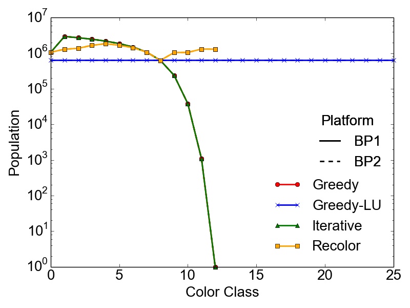
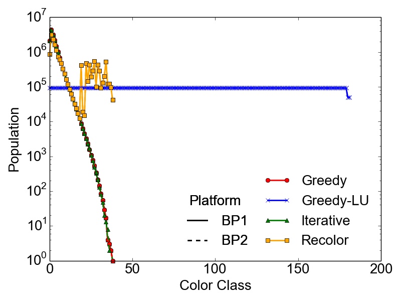
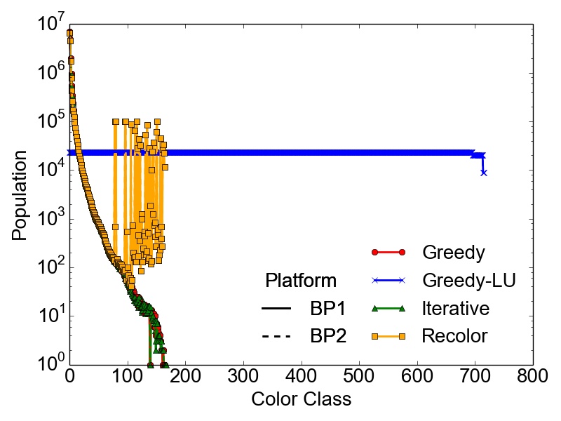
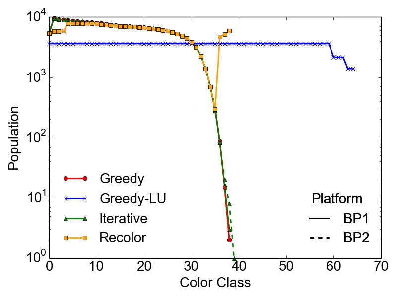
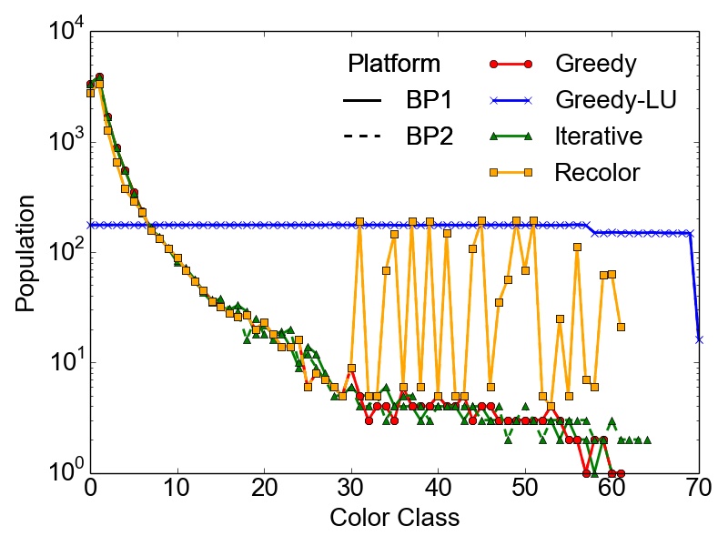
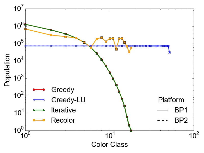
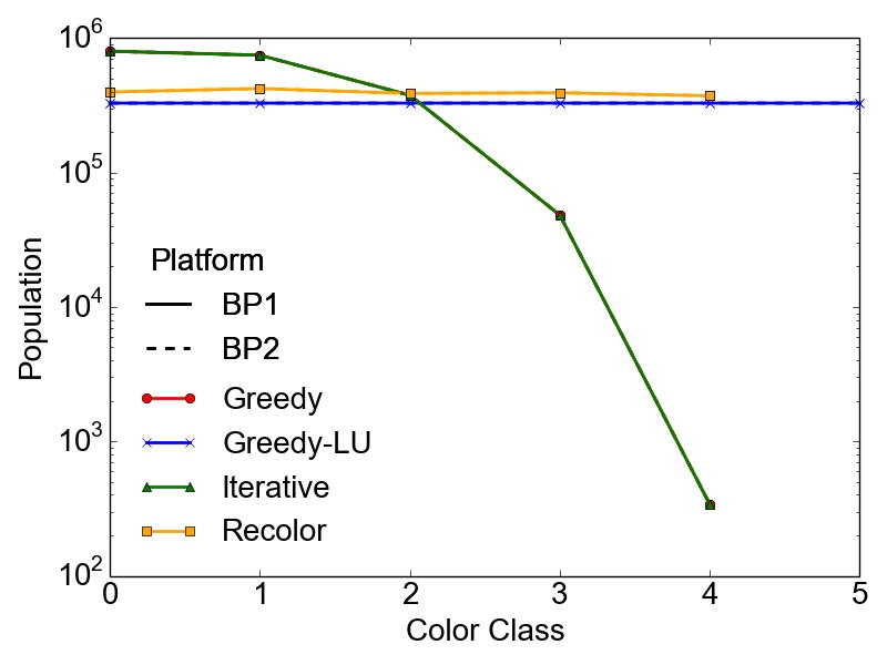
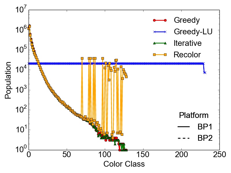
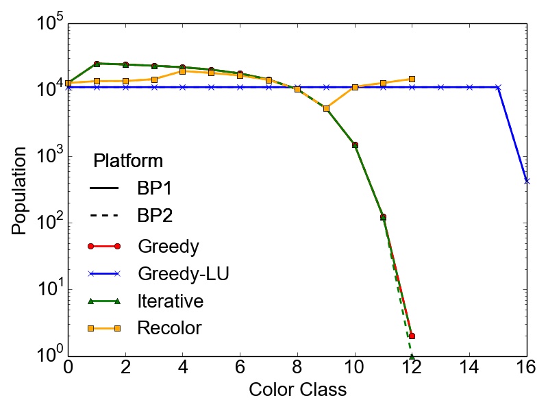
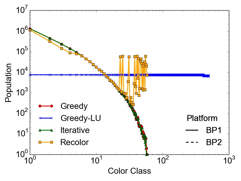
However, the maximum number of colors \(k\) used to compute a feasible coloring of a graph \(G(V,E)\) is not enough to properly quantify the different results obtained with the presented algorithms. It is also necessary to evaluate the population of the color classes, especially if the coloring is done with respect to a potentially subsequent parallel computation of the tasks represented by the created independent sets. In this case, highly skewed color classes could lead to potentially harmful computational bottlenecks regarding the parallel performance of an application. Therefore, Table 3.5 contains the RSDs (Equation 2.13) of the population of the color classes for the set of test graphs on the different BPs. Additionally, Figure 3.2 depicts the population of the color classes obtained on both BPs for the set of test graphs.
As expected, the presented data proves that in most cases the most optimal balancing of the color populations is obtained using the Greedy-LU algorithm. For this algorithm, the RSD over the whole set of test graphs is in the worst case 38%, observed for the RoadNet-CA graph. Although, this result seems to indicate a rather non-optimal population, the simple reason is that for this particular graph, the number of colors is quite small, i.e., seven. This affects also the population of the specific classes, yielding the result of a single color class creating this deviation. The RoadNet-CA and the RMAT-ER graph are instances of the test set, where the Recolor algorithm outperforms the Greedy-LU algorithm with respect to balanced color classes. Also for the Trigate_5 graph, modeling a semiconductor device, the Recolor algorithm delivers well balanced color classes using fewer colors than the Greedy-LU algorithm.
Additionally, the success of the Recolor approach is heavily influenced by the vertex degree distribution of the graph and the initial coloring. Due to these constraints, large differences in population numbers occur which are
observable, for example, in the
soc-LiveJournal1, the Wikipedia, and the RMAT-B graph. On the contrary, the skewed populations in the RMAT-G graph are balanced using Recolor, while keeping the number of used colors \(k\) way below the balanced
competitor Greedy-LU. Nevertheless, the depicted populations and the shown RSDs prove that the overall initial differences in color populations resulting from the greedy approach are alleviated (e.g., cit-Patents or BMW3_2
populations).
For lower color classes Recolor results in the same population as Greedy, since it tries to move vertices only from higher (populated) to lower (populated) color classes. A fact that also needs to be taken into account is that with this algorithm the nearly optimal number of colors \(k\) applied with the initial Greedy coloring is not increased, a possibly important fact regarding parallelization methods for different computational problems, where a single lowly populated color class could have a severe performance impact. The RSDs indicate also that the populations obtained with Greedy and Iterative are similar, even for the maximum number of threads applied with the latter algorithm. Hence, a parallel Greedy coloring approach has no practical influence on the final population of the color classes, except possible faster runtimes. This proves the quality of the results obtained using the evaluated parallel approach.
| Graph | Platform | Greedy | Greedy-LU | Iter 1T | Iter MT | Recolor |
| RMAT-ER | BP1 | 72.11 | 13.0 | 72.11 | 72.11 | 21.1 |
| BP2 | 80.43 | 0.0 | 80.43 | 80.43 | 24.31 | |
| RMAT-G | BP1 | 216.04 | 11.0 | 216.04 | 212.46 | 140.19 |
| BP2 | 223.02 | 5.0 | 223.02 | 216.04 | 148.75 | |
| RMAT-B | BP1 | 683.26 | 0.0 | 683.26 | 683.26 | 646.48 |
| BP2 | 666.93 | 4.0 | 666.93 | 673.1 | 629.29 | |
| BMW3_2 | BP1 | 51.4 | 13.0 | 51.4 | 51.4 | 37.5 |
| BP2 | 48.23 | 14.0 | 48.23 | 51.36 | 33.74 | |
| ca-HepPh | BP1 | 325.22 | 7.0 | 325.22 | 337.89 | 260.05 |
| BP2 | 348.37 | 12.0 | 348.37 | 356.72 | 287.0 | |
| cit-Patents | BP1 | 180.8 | 0.0 | 180.8 | 180.8 | 69.5 |
| BP2 | 187.31 | 11.0 | 187.31 | 187.31 | 78.81 | |
| RoadNet-CA | BP1 | 85.16 | 38.0 | 85.16 | 85.16 | 4.06 |
| BP2 | 85.18 | 0.0 | 85.18 | 85.18 | 4.04 | |
| soc-LiveJournal1 | BP1 | 509.19 | 3.0 | 509.19 | 513.37 | 464.91 |
| BP2 | 515.35 | 6.0 | 515.35 | 515.35 | 471.54 | |
| Trigate_5 | BP1 | 66.46 | 13.0 | 66.46 | 66.45 | 25.05 |
| BP2 | 66.38 | 24.0 | 66.38 | 66.38 | 24.93 | |
| Wikipedia | BP1 | 368.66 | 7.0 | 368.66 | 378.76 | 305.18 |
| BP2 | 372.1 | 4.0 | 372.1 | 372.09 | 309.18 | |
Table 3.5: RSDs of the various test graphs colored with different graph coloring algorithms. For the Iterative algorithm (Iter) the results obtained using one thread (1T) and the maximum available number of threads (MT) on the specific BP are shown.
(g) RoadNet-CA
(h) soc-LiveJournal1
(i) Trigate_5
(j) Wikipedia
Figure 3.2: Continued.
3.2.4 Performance Analysis
The aim of this section is to give an overview and analysis of the strong scaling capabilities, i.e., scaling for a fixed problem size, of the investigated graph coloring algorithms. Hence, the algorithms are evaluated on both BPs with the entire set of test graphs. The obtained runtimes are depicted in Table 3.6 and the speedups for the test graphs in Figure 3.3.
In most cases, the shared-memory parallel Iterative coloring algorithm shows the best performance with respect to the total runtimes. Nevertheless, for the ca-HepPh graph the Greedy algorithm outperforms all other algorithms on both BPs. This is due to the specific properties of this graph, i.e., its rather small number of graph vertices and their degree distribution. These results show that for small graphs the serial Greedy algorithm still proves to be a proper option for solving the graph coloring problem in terms of computational performance. The superior runtimes obtained with Greedy on BP1 for the RoadNet-CA and the Trigate_5 graph result from the small number of vertex degrees. Additionally, the total number of vertices for the latter graph is rather low compared to the RoadNet-CA graph. Although the RoadNet-CA graph has about 2 million graph vertices, the performance of both parallel algorithms suffers from the small maximum vertex degree of \(\Delta G = 8\).
Regarding the RMAT graphs, it is shown that the runtimes for the different algorithms vary widely, although the graphs have the same number of graph vertices. This is due to the fact that the degree distributions of the RMAT graphs are different, where some of them have many local maxima and minima, resulting in a higher difficulty for the graph coloring algorithms to compute a feasible solution.
The obtained runtimes for the Wikipedia graph, where the Greedy algorithm on BP1 performs the best, show that not only the graph properties or the algorithms themselves influence the performance results, but also the specific hardware architecture of the BPs. As it is shown in Table 3.6, the runtimes on BP1 for the serial algorithms are superior than on BP2, due to the higher clock frequency. Nevertheless, the high number of available cores on BP2 results in faster runtimes than on BP1 using the maximum number of threads. However, these results are obtained using 64 threads, which is four times more than on BP1. Regarding the Recoloring algorithm, the runtimes show that, due to Amdahl’s law (Equation 2.23), the serial initial coloring step limits the potential performance gain of the parallel recoloring step.
| Graph | Greedy | Greedy-LU | Iter 1T | Iter MT | Rec 1T | Rec MT |
| RMAT-ER | 7.70 | 14.24 | 30.01 | 3.57 | 30.41 | 24.48 |
| 53.59 | 57.68 | 102.05 | 2.54 | 80.87 | 51.29 | |
| RMAT-G | 23.01 | 48.28 | 18.85 | 11.17 | 23.58 | 11.43 |
| 63.00 | 152.65 | 89.51 | 2.60 | 39.10 | 2.84 | |
| RMAT-B | 6.09 | 169.78 | 231.38 | 18.96 | 19.68 | 11.83 |
| 50.14 | 478.69 | 562.62 | 11.17 | 88.08 | 57.57 | |
| BMW3_2 | 0.09 | 0.41 | 0.29 | 0.05 | 0.17 | 0.12 |
| 0.81 | 1.13 | 1.34 | 0.04 | 1.10 | 0.87 | |
| ca-HepPh | 0.002 | 6.902 | 0.006 | 0.009 | 0.002 | 0.007 |
| 0.007 | 0.041 | 0.041 | 0.010 | 0.019 | 0.019 | |
| cit-Patents | 0.84 | 4.36 | 2.25 | 0.70 | 2.53 | 1.89 |
| 5.37 | 13.20 | 8.93 | 0.51 | 9.99 | 5.89 | |
| RoadNet-CA | 0.35 | 0.66 | 0.44 | 0.36 | 0.51 | 0.48 |
| 1.40 | 2.33 | 2.13 | 0.27 | 2.03 | 1.60 | |
| soc-LiveJournal1 | 2.96 | 17.67 | 13.56 | 1.28 | 5.10 | 2.76 |
| 14.71 | 53.82 | 46.46 | 1.03 | 28.03 | 15.44 | |
| Trigate_5 | 0.046 | 0.145 | 0.094 | 0.048 | 0.081 | 0.051 |
| 0.333 | 0.416 | 0.585 | 0.038 | 0.456 | 0.334 | |
| Wikipedia | 1.85 | 24.71 | 89.55 | 6.87 | 3.82 | 2.31 |
| 10.83 | 69.33 | 168.45 | 6.80 | 16.01 | 10.88 | |
Table 3.6: Runtimes (in seconds) of the different algorithms for the set of test graphs, where Iter and Rec denote Iterative and Recolor, respectively, with one thread (1T) and the maximum number of available threads (MT). Results for BP1 are shown in the top row, for BP2 on the bottom row for each graph. The runtime of the best performing algorithm is given in bold.
In addition to the runtimes also the strong scaling behavior of the algorithms is evaluated. The speedups for both BPs are shown in Figure 3.3. For the Recolor algorithm only the speedup of the actual parallel recoloring step is depicted, omitting the serial initial coloring of the graph. The best speedup is observed for the Iterative algorithm on the soc-LiveJournal1, the Wikipedia, and the RMAT-B graph on BP1. Similar results were obtained on the second BP, with the Iterative algorithm showing partially better speedup on the RMAT-ER graph than on the RMAT-B. In most cases the speedup curves for the Iterative algorithm show a kink at eight and 32 threads on BP1 and BP2, respectively: On the first BP only eight cores are available per socket, thus, the speedup due to the random memory accesses is deteriorated using the maximum number of available cores as both sockets are utilized. However, in some cases the speedup is linear, e.g., RMAT-B and Wikipedia, proving that the Iterative algorithm can in principle scale well. Nevertheless, in general, NUMA effects and limited memory bandwidth restrict the potential maximum speedup. Regarding the Recolor algorithm, the presented data indicate that the speedup is usually below the Iterative algorithm and in case of the ca-HepPh graph even below one. The reason for this behavior is, that the Recolor algorithm does not introduce new color classes in the recoloring step. Thus, it only moves vertices from highly to lowly populated color classes, resulting in insufficient workload per thread for some color classes, which subsequently limits the potential speedup.
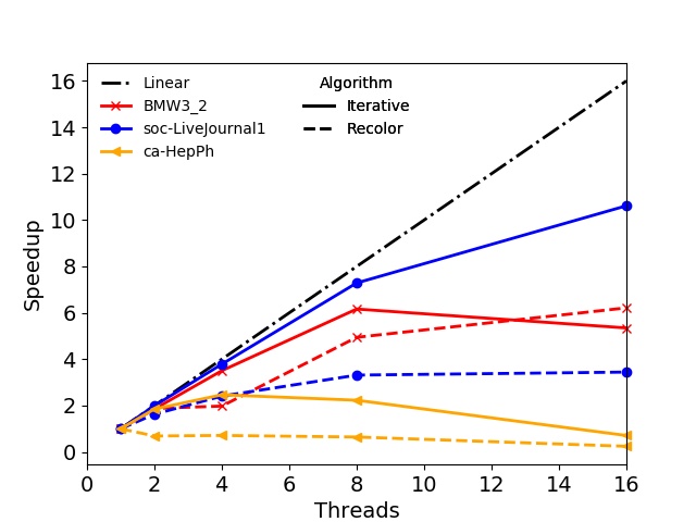
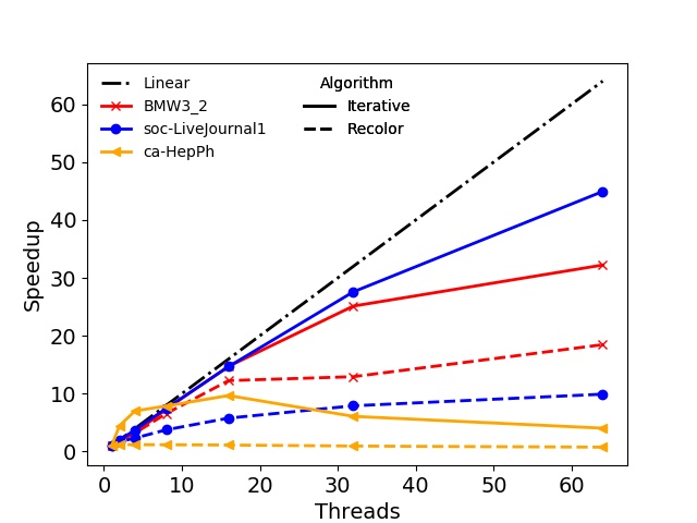
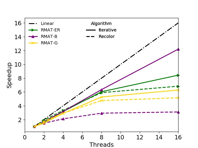
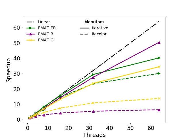
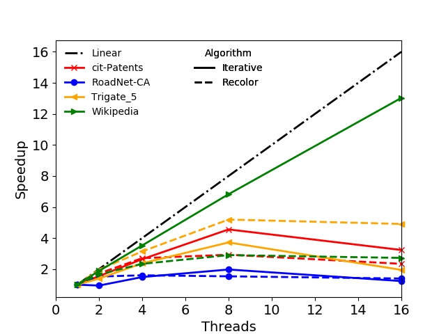
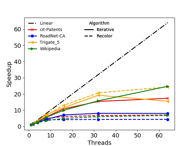
Figure 3.3: Speedups obtained with the shared-memory parallel algorithms for the test graphs using the two benchmarking platforms. The three figures in the left column show results for BP1, the figures in the right column for BP2. For the Recolor algorithm only the speedups of the actual recoloring step are shown.
The presented speedup data show, that the utilization of parallel graph coloring approaches is able to reduce the necessary computation time. However, depending on the specific hardware and the actual properties of the graph to be colored, the obtainable speedup can be limited or even decrease with higher thread counts. This is, for example, the case with the ca-HepPh graph. Nevertheless, there are test graphs where the strong scaling capabilities are very well utilized yielding good speedup, e.g., a speedup about 12 and 50 for the RMAT-B graph on BP1 and BP2, respectively.
An interesting behavior has been observed for the ca-HepPh graph colored with the Iterative algorithm on BP2: For thread counts below eight the obtained speedup is superlinear. To explain this, it has to be noted that the worst-case algorithmic complexity of the Greedy coloring approach is \(\mathcal {O}(n^2)\). However, in most cases the complexity of the algorithm is linear, i.e., \(\mathcal {O}(n \log {} n)\) [33]. If now \(N\) threads are utilized for the parallel algorithm, its speedup can be described as [129]
\( \seteqsection {3} \) \( \seteqnumber {6} \)
\begin{equation} \frac {n \log (n)}{\frac {n}{N} \log (\frac {n}{N})} = N \frac {1}{1-\frac {\log (N)}{\log (N)}}. \label {eq:coloring:superlinear} \end{equation}
Since the fraction on the right-hand side is greater than one, the observed speedup for \(N\) threads can be superlinear. In reality, however, this rarely happens, as non-perfect load balancing of the problem or memory latency jeopardize this potential superlinearity.
3.3 Summary and Conclusion
The chapter introduced different approaches of solving the graph coloring problem, ranging from exact to approximative solutions. It was discussed why the approximative approach is often preferred: Shorter runtimes with nearly optimal solution quality. In most computational disciplines it is not necessary to compute an exact solution, but it is rather important to efficiently generate approximative solutions.
To evaluate the behavior and solution quality of the chosen algorithms, benchmarks on two different platforms were performed using a set of test graphs. These graphs included artificially generated graphs, using the RMAT scheme, as well as graphs modeling real world problems in engineering, like the Trigate_5 graph, or social sciences, e.g., soc-LiveJournal1. The benchmarks covered solution properties as the maximum number of used colors or the population of the color classes, in addition to the parallel performance of each algorithm.
It was shown that recently presented shared-memory parallel algorithms offer advantages regarding runtimes, while simultaneously creating similar coloring results as serial approaches. Nevertheless, the goal of creating equally or nearly equally balanced color classes remains a difficult challenge, as proven by the large runtimes of the Greedy-LU algorithm. Parallel approaches trying to alleviate this skewness are limited such that no new colors are to be introduced, therefore, limiting the ways of reducing skewed color populations. However, the benefit of less number of colors persists for the Recolor algorithm, which can be an advantage with respect to load balancing of problems occurring in computational science and engineering, where the graph vertices typically represent parts of computationally difficult workloads. Furthermore, the presented graph coloring algorithms build the basis for the shared-memory parallel approaches presented in the Chapters 4 and 5.