1 Introduction and Motivation

With the increasing complexity of modern semiconductor devices, it becomes more and more important to not only evaluate different device designs but also to increase the efficiency and accuracy of the underlying processing and fabrication steps. Due to astonishing technological developments in the semiconductor industry as well as in research and due to ever shorter production cycles of new devices, there is not always enough time or funding to experimentally address all of the occurring challenges [1]. Thus, computer simulations play a major role in the modern semiconductor industry, replacing a fair amount of expensive and time-consuming experimental evaluations of new processes and devices [2].

This important use case of the aforementioned computer simulations is called Technology Computer-Aided Design (TCAD). TCAD is used to conduct computer simulations aiming at modeling and predicting the fabrication and operation of semiconductor devices and circuits. It is widely used in research and industry to gain a deeper understanding of the implications of potential new technologies, to evaluate new processing techniques [3], [4], and to evaluate new device designs [5], [6], [7], [8]. In general, the field of TCAD can be split up into three different branches: Process TCAD, Device TCAD, and Circuit TCAD (Figure 1.1) [9].

In Process TCAD, the overall goal is to model the various processing methods, which are necessary to fabricate a semiconductor device. Examples are photolithography, etching, deposition, and doping [10]. The research within the field of Process TCAD focuses primarily on the investigation of the underlying physical processes to enhance the accuracy of the predictions obtained through process simulations. Thus, a lot of effort goes into modeling these fundamental physical processes. The computational demands of these models are a key factor for their application in TCAD simulations, requiring the development of computationally efficient numerical simulation methods. Therefore, models approximating the required processes and properties while simultaneously reducing the computational effort are of major interest.

Eventually, Process TCAD yields geometries and physical properties, e.g., doping profiles, which serve as input data for a potential subsequent Device TCAD investigation.

Device TCAD describes computer simulations aiming at predicting the electrical characteristics of a semiconductor device. The simulations base on physical models, using the input provided by prior process simulations. The determination of the device characteristics plays a significant role to gain a better understanding of the electrical behavior and to further improve their reliability. In the semiconductor industry, Device TCAD is used to speedup the development cycles for new technologies while simultaneously reducing the required resources. In turn, the derived electrical characteristics of a device are used by Circuit TCAD simulations.

Circuit TCAD aims at predicting the behavior and interplay of several semiconductor devices, such as resistors, transistors, and diodes. The typical use case for these type of TCAD simulations is the design and evaluation of circuits prior to their actual large-scale fabrication.

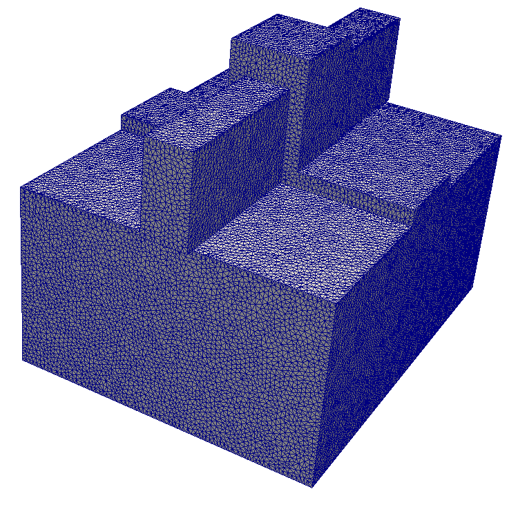
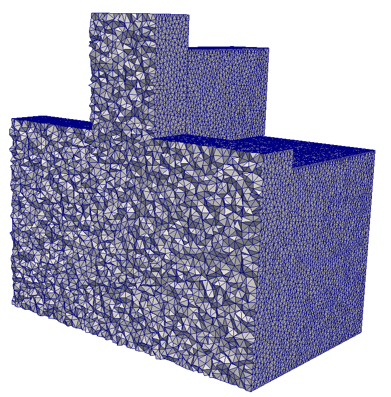
Figure 1.2 shows an overview of the different steps occurring in a typical TCAD workflow. Very typical in Process and Device TCAD is the use of finite element (FEM) [11] or finite volume methods (FVM) [12] to simulate the fabrication of a device and the resulting device’s electrical characteristics [13], [14]. In general, FEM and FVM are used to solve partial differential equations (PDEs), which are the mathematical foundation used to describe the investigated physical processes [15]. A PDE requires a spatial discretization of the simulation domain, commonly known as mesh, together with boundary conditions modeling the exchanges with the environment (e.g., current). Figures 1.3 and 1.4 depict two types of meshes used, for example, in Process TCAD and Device TCAD. The first mesh is a 2D mesh representing a surface during the simulation of an etching process. The second mesh is a 3D tetrahedral mesh modeling a semiconductor device, i.e., a FinFET [16].

In Process TCAD, surface meshes (e.g., Figure 1.3) are used, for example, to simulate an etching process. A typical challenge is that these meshes have an unnecessarily high resolution, i.e., too many surface mesh elements which are not required to efficiently describe the surface geometry. Such inefficiencies lead to considerable computational overhead when calculating Process TCAD relevant distributions on these over-resolved surfaces [17]: The mesh resolution has a major influence on the runtime of the simulation. One way to increase the computational performance is to adapt the elements in the mesh (e.g., reducing the number of mesh elements) or to choose only a suitable subset of the elements for the actual calculations, while keeping the actual mesh untouched. Both methods in essence represent mesh adaptation steps, see Figure 1.2. As indicated by the several timesteps shown in Figure 1.3, the surface evolution during a process simulation can potentially require a mesh adaptation step in every timestep: The evolution of the surface changes the geometry, in turn requiring an surface mesh updates to avoid mesh inconsistencies (e.g., element overlaps and deterioration of element quality). This is particularly the case if the etching simulation is based on an implicit surface representation, where the explicit surface mesh is extracted in every single timestep [17]. Hence, the performance of the mesh adaptation step has a major influence on the overall simulation performance [18].

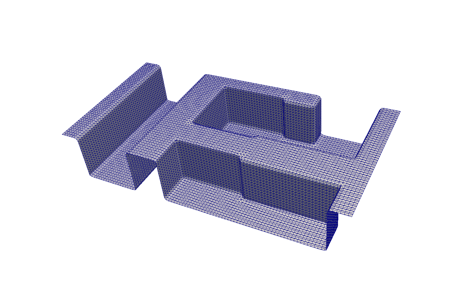
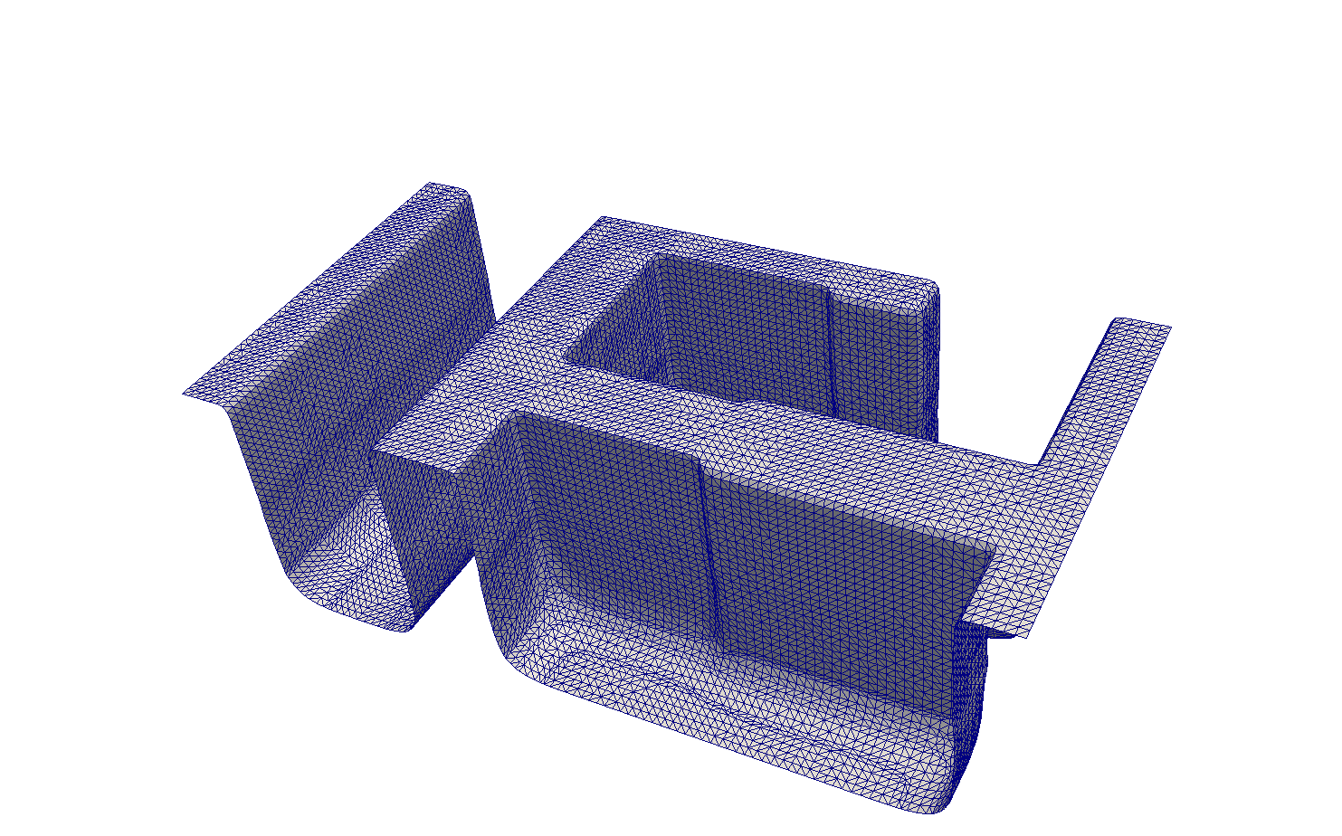
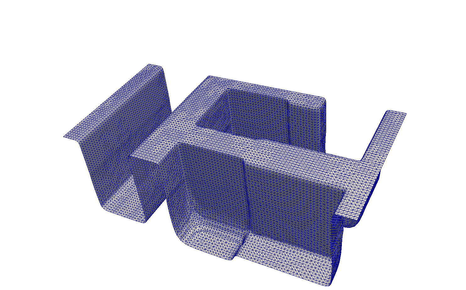
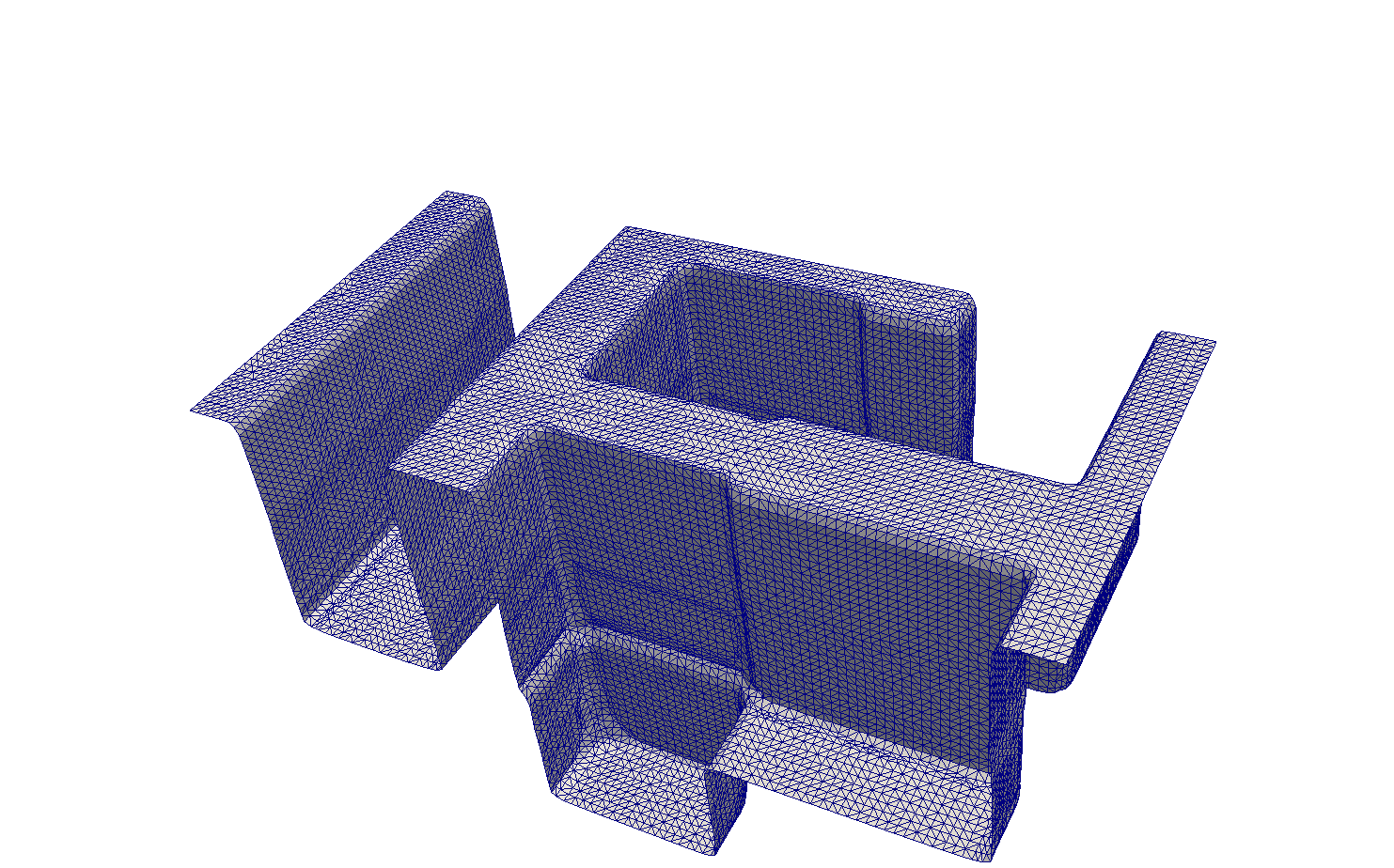
In Device TCAD the meshes represent electrical devices, e.g., FinFETs (see Figure 1.4). An accurate representation of material interfaces as well as higher resolutions in specific regions of interest commonly guide a potential mesh adaptation process. For example, the properties of FinFETs, e.g., doping and charge carrier distributions, are simulated based on a suitable mesh representing the device [19], [20], [21]. This potential mesh adaptation step is indicated in green in the general TCAD workflow in Figure 1.2. Additionally, it is possible that the geometry of the physical model changes in certain scenarios, e.g., deformation due to volume stresses, bending, or compression of the modeled device, requiring an adaptation of the mesh [22]. Here, mesh adaptation proves to be one option to avoid deteriorated geometries and to enable dynamic regions of interest in a device.

However, in Circuit TCAD no meshes are needed as the simulated circuit is abstracted using compact models for individual devices, which are derived from the simulated electrical characteristics obtained by Device TCAD.

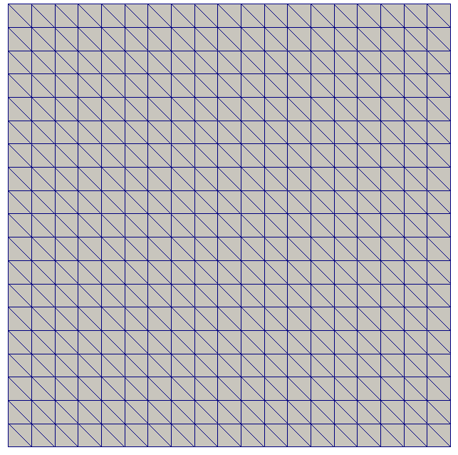
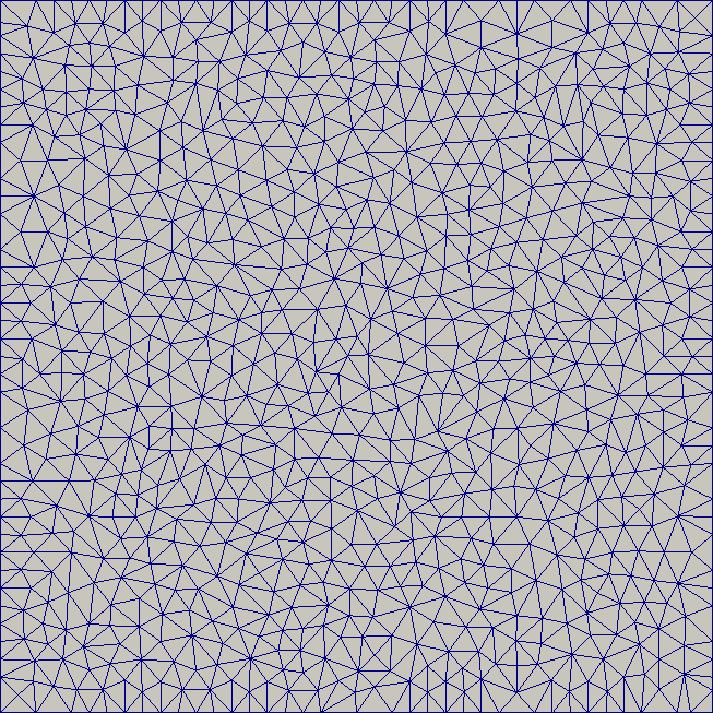
Typically, two fundamentally different mesh types for numerical simulations exist: (1) a structured and (2) an unstructured mesh (see Figure 1.5). The first denotes a discretization of the simulation domain using a set of indices with the number of indices being equal to the number of space dimensions, e.g., three for three dimensions. In such a structured mesh the vertices are labeled using these indices such that the indices of adjacent vertices differ at most by unity. Thus, each element in a structured mesh is defined via a unique set of indices and due to its regular structure every mesh entity, i.e., vertices, edges, and elements, has the same number of adjacent entities except on the mesh boundary [23]. Therefore, adjacency information does not need to be stored explicitly as it is implicitly available via using basic arithmetic. However, it is quite difficult to model complex geometries using a structured grid, requiring increased mesh resolutions which due to the structured mesh condition translates into over-proportional mesh sizes (in terms of numbers of elements). To overcome this issue, unstructured meshes are used, which explicitly store the adjacency information of vertices and elements. Thus, algorithms for building up the required information and for retrieving adjacency information when necessary have to be devised. This increases the computational complexity as well as the algorithm complexity, for example, for mesh refinement. In general, though, unstructured meshes enable to increase the resolution only in specific regions of interest, requiring considerable less mesh elements to model complex geometries as compared to structured meshes. Overall, considering complex geometries unstructured meshes yield faster runtimes with the same level of accuracy for FEM/FVM based simulations [23].

The efficiency and accuracy of numerical studies are heavily influenced by the resolution of the mesh. As previously indicated, it is often necessary to locally or globally adapt the mesh. However, due to the potentially large number of elements contained in an initial mesh (e.g., generated by marching cubes algorithms [24], applied to implicitly defined surface meshes, as are typical for Process TCAD simulations), the mesh adaptation step can become a critical computational bottleneck in a simulation pipeline (see Figure 1.2).

For example, this bottleneck becomes particularly severe if the mesh adaptation has to be conducted several times to derive a proper resolution in specific regions of interest, or if the adaptation has to be done after each solution step of a simulation pipeline in order to correctly update the mesh according to changed geometries or mesh-critical quantity distributions [17].

One approach for improving the performance of any computational problem is the use of parallel computers or high-performance computing clusters. Commonly, high-performance computing clusters consist of several hundreds or thousands of compute nodes¹ forming a distributed-memory system. In a distributed-memory system, independent processors with exclusive memory are connected via a network interface (Figure 1.6a). Therefore, it is necessary to decompose the computational problem at hand into several smaller parts, where each part is assigned to a specific processor.

With the ongoing down-scaling of transistors, processor vendors are able to pack more and more processor cores into their processor packages using a shared-memory architecture. This ongoing and fast-pacing development results in an ever-growing capacity of on-node parallelism and provides ample of parallel resources already on a single node (Figure 1.6b) [25].

Despite the promising performance gain of modern shared-memory systems, the increasing parallel resources introduce challenges in algorithm and data structure designs. In order to optimally exploit the potential of shared-memory parallel computers, the parallel algorithm and data structures need to be carefully designed and implemented. A critical aspect is the simultaneous access and manipulation of data stored in memory: Concurrent data operations need to be considered for efficient, correct, and robust implementations (see race condition [26]). Hence, various methods have been proposed in the past in order to tackle the challenge of safely synchronizing the parallel processing of data in shared-memory parallelized applications. For example, to guarantee concurrent read and write operations on a shared resource, e.g., data stored in memory, the general concept of critical sections can be used to define sections of code in a program, where only a single thread is allowed to execute the specific operations. Every other thread has to wait before it can execute the same code section (i.e., accessing the critical resource), thus avoiding data races. Nevertheless, a critical section can lead to scenarios where a thread is waiting for a shared resource to be freed, but this resource never becomes available [26].

Regardless of the parallelization approach, the fundamental challenge is to maximize the degree of parallelization to ultimately maximize the achieved speedup, when developing a parallel algorithm. One approach for organizing the operations to be conducted in parallel stems from the field of graph theory. The main idea is to decompose a computational problem into independent sets using a technique called graph coloring. The rationale behind is that, the created sets can be safely processed in parallel without running into any synchronization issues, e.g., data races. Numerous examples of applications requiring a guarantee on safe parallel execution exist, including linear algebra [27], community detection [28], and mesh adaptation [29], [30], [31].

Since graphs can generally model any relationships between any kind of objects, they are widely used in different fields of research, including social sciences, electrical engineering, and computational science [32], [33], [34]. Commonly, the idea behind any graph coloring algorithm is to assign each graph vertex a color such that no two neighboring vertices have an identical color. Combining all vertices with the same color into a dedicated set subsequently yields independent sets of vertices with different colors. Figure 1.7 shows an example graph consisting of six vertices together with a potential coloring using four different colors. This example shows that the vertices 1 and 5, as well as 3 and 6, represent two different independent sets, each including two vertices. The remaining two vertices, i.e., 2 and 4, are also contained in different independent sets.

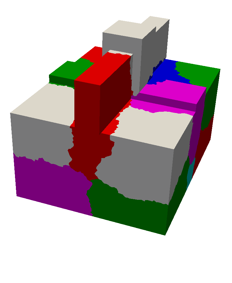
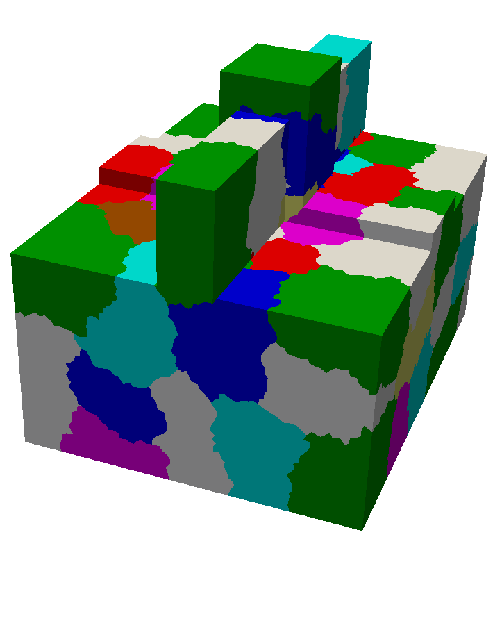
Considering mesh adaptation, the initial mesh can be split into several partitions, which are subsequently assigned to independent sets (see Figure 1.8). These independent sets, denoted by different colors, can then be processed in parallel, e.g., using a mesh adaptation algorithm without facing any synchronization issues on the partition boundaries [31]. For example, each graph vertex in Figure 1.7 potentially represents such a partition. If operations on the mesh are conducted in parallel, for example, on the partitions represented by the graph vertices 1 and 2, it can be guaranteed that they do not share any mesh elements. This prevents potential data races or inconsistencies on the partition boundaries and thus drastically simplifies the actual parallelization algorithm and in turn promises higher parallel efficiency.

In general, the graph coloring problem (i.e., finding the minimum number of colors for coloring the graph) is NP-complete [35]. In most cases it is not necessary to solve the graph coloring problem such that the number of colors is minimized: A non-optimal solution is often sufficient [33]. For example, if the coloring of the mesh partitions is dominating the overall runtime, a potential benefit of subsequent parallel operations is jeopardized. It is obvious that a parallel approach yields several challenges which have to be resolved to obtain a proper coloring solution. For example, a parallel graph coloring algorithm has to ensure that color clashes, i.e., two adjacent graph vertices having the same color, are either prevented or resolved. Another important aspect is the final number of vertices in each independent set. If colors have a large deviation in their population, i.e., highly different number of vertices per color, it is possible that subsequent parallel computations cannot exploit the available parallel resources due to load imbalancing. Therefore, it is highly desirable to balance the color populations ensuring the performance gain obtained through parallelization [28].

1.1 Research Goals

Considering the above discussions, this work focuses on efficiently utilizing the available on-node parallelism on modern computer architectures for mesh adaptation using shared-memory parallel graph coloring algorithms. Furthermore, methods from both graph theory and mesh adaptation are utilized to increase the performance of Process TCAD simulations. The conducted research focuses especially on the following topics:

• • Evaluation of available serial and shared-memory parallel graph coloring algorithms.

• • Development of a coarse-grained shared-memory parallel mesh adaptation framework based on graph coloring algorithms, which is capable of applying available serial meshing algorithms in parallel.

• • Implementation of a partitioning approach for surface meshes in order to enhance the computational performance in semiconductor etching simulations.

1.2 Research Setting

The research presented in this work was conducted within the scope of the Christian Doppler Laboratory for High Performance Technology Computer-Aided Design. The Christian Doppler Association funds cooperations between companies and research institutions pursuing application-orientated basic research. In this case, the cooperation was established between the Institute for Microelectronics at the TU Wien and Silvaco Inc., a company developing and providing electronic device automation and TCAD software tools.

1.3 Thesis Outline

In the following a brief overview of the structure of the thesis is given:

Chapter 2 provides a formal introduction into the topics of graphs and graph theory as well as meshing and mesh adaptation. The chapter ends with an overview of modern computer architectures and parallel processing/programming methods.

Chapter 3 introduces the distance-1 graph coloring problem commonly found in computational science and engineering. An overview of different approaches of solving the graph coloring problem is given, including exact and approximative algorithms. A particular focus is on available state-of-the-art general-purpose shared-memory parallel coloring algorithms for balanced and unbalanced graph coloring. The chapter continues with an evaluation of various algorithms regarding coloring quality and computational performance.

Chapter 4 investigates shared-memory parallel mesh adaptation frameworks. In particular, the requirements and challenges of such a framework are discussed followed by an overview of available shared-memory parallel meshing frameworks. Finally, a novel coarse-grained shared-memory parallel mesh adaptation framework utilizing available serial algorithms in parallel, based on mesh partitioning and graph coloring, is presented together with a discussion of the included software libraries.

Chapter 5 presents a related method to improve the performance of a multi-material Process TCAD etching simulation. The approach is based on a partitioning of the surface mesh conducted by creating a suitable subset of the surface mesh elements. The developed method outperforms a full evaluation using all mesh elements and simultaneously keeping the introduced error quite small.

Chapter 6 gives a brief summary and concludes with ideas for future work.